difference between research questions and null hypothesis

• Customer Reviews
• Extended Essays
• IB Internal Assessment
• Theory of Knowledge
• Literature Review
• Dissertations
• Essay Writing
• Research Writing
• Assignment Help
• Capstone Projects
• College Application
• Online Class

Research Questions vs Hypothesis: What’s The Difference?

by  Antony W

August 1, 2024

You’ll need to come up with a research question or a hypothesis to guide your next research project. But what is a hypothesis in the first place? What is the perfect definition for a research question? And, what’s the difference between the two?

In this guide to research questions vs hypothesis, we’ll look at the definition of each component and the difference between the two.

We’ll also look at when a research question and a hypothesis may be useful and provide you with some tips that you can use to come up with hypothesis and research questions that will suit your research topic . 

Let’s get to it.

What’s a Research Question?

We define a research question as the exact question you want to answer on a given topic or research project. Good research questions should be clear and easy to understand, allow for the collection of necessary data, and be specific and relevant to your field of study.

Research questions are part of heuristic research methods, where researchers use personal experiences and observations to understand a research subject. By using such approaches to explore the question, you should be able to provide an analytical justification of why and how you should respond to the question. 

While it’s common for researchers to focus on one question at a time, more complex topics may require two or more questions to cover in-depth.

When is a Research Question Useful? 

A research question may be useful when and if: 

• There isn’t enough previous research on the topic
• You want to report a wider range out of outcome when doing your research project
• You want to conduct a more open ended inquiries 

Perhaps the biggest drawback with research questions is that they tend to researchers in a position to “fish expectations” or excessively manipulate their findings.

Again, research questions sometimes tend to be less specific, and the reason is that there often no sufficient previous research on the questions.

What’s a Hypothesis? 

A hypothesis is a statement you can approve or disapprove. You develop a hypothesis from a research question by changing the question into a statement.

Primarily applied in deductive research, it involves the use of scientific, mathematical, and sociological findings to agree to or write off an assumption.

Researchers use the null approach for statements they can disapprove. They take a hypothesis and add a “not” to it to make it a working null hypothesis.

A null hypothesis is quite common in scientific methods. In this case, you have to formulate a hypothesis, and then conduct an investigation to disapprove the statement.

If you can disapprove the statement, you develop another hypothesis and then repeat the process until you can’t disapprove the statement.

In other words, if a hypothesis is true, then it must have been repeatedly tested and verified.

The consensus among researchers is that, like research questions, a hypothesis should not only be clear and easy to understand but also have a definite focus, answerable, and relevant to your field of study. 

When is a Hypothesis Useful?

A hypothesis may be useful when or if:

• There’s enough previous research on the topic
• You want to test a specific model or a particular theory
• You anticipate a likely outcome in advance 

The drawback to hypothesis as a scientific method is that it can hinder flexibility, or possibly blind a researcher not to see unanticipated results.

Research Question vs Hypothesis: Which One Should Come First 

Researchers use scientific methods to hone on different theories. So if the purpose of the research project were to analyze a concept, a scientific method would be necessary.

Such a case requires coming up with a research question first, followed by a scientific method.

Since a hypothesis is part of a research method, it will come after the research question.

Research Question vs Hypothesis: What’s the Difference? 

The following are the differences between a research question and a hypothesis.

We look at the differences in purpose and structure, writing, as well as conclusion. 

Research Questions vs Hypothesis: Some Useful Advice 

As much as there are differences between hypothesis and research questions, you have to state either one in the introduction and then repeat the same in the conclusion of your research paper.

Whichever element you opt to use, you should clearly demonstrate that you understand your topic, have achieved the goal of your research project, and not swayed a bit in your research process.

If it helps, start and conclude every chapter of your research project by providing additional information on how you’ve or will address the hypothesis or research question.

You should also include the aims and objectives of coming up with the research question or formulating the hypothesis. Doing so will go a long way to demonstrate that you have a strong focus on the research issue at hand. 

Research Questions vs Hypothesis: Conclusion 

If you need help with coming up with research questions, formulating a hypothesis, and completing your research paper writing , feel free to talk to us. 

About the author 

Antony W is a professional writer and coach at Help for Assessment. He spends countless hours every day researching and writing great content filled with expert advice on how to write engaging essays, research papers, and assignments.

Ohio State nav bar

The Ohio State University

• BuckeyeLink
• Find People
• Search Ohio State

Research Questions & Hypotheses

Generally, in quantitative studies, reviewers expect hypotheses rather than research questions. However, both research questions and hypotheses serve different purposes and can be beneficial when used together.

Research Questions

Clarify the research’s aim (farrugia et al., 2010).

• Research often begins with an interest in a topic, but a deep understanding of the subject is crucial to formulate an appropriate research question.
• Descriptive: “What factors most influence the academic achievement of senior high school students?”
• Comparative: “What is the performance difference between teaching methods A and B?”
• Relationship-based: “What is the relationship between self-efficacy and academic achievement?”
• Increasing knowledge about a subject can be achieved through systematic literature reviews, in-depth interviews with patients (and proxies), focus groups, and consultations with field experts.
• Some funding bodies, like the Canadian Institute for Health Research, recommend conducting a systematic review or a pilot study before seeking grants for full trials.
• The presence of multiple research questions in a study can complicate the design, statistical analysis, and feasibility.
• It’s advisable to focus on a single primary research question for the study.
• The primary question, clearly stated at the end of a grant proposal’s introduction, usually specifies the study population, intervention, and other relevant factors.
• The FINER criteria underscore aspects that can enhance the chances of a successful research project, including specifying the population of interest, aligning with scientific and public interest, clinical relevance, and contribution to the field, while complying with ethical and national research standards.

• The P ICOT approach is crucial in developing the study’s framework and protocol, influencing inclusion and exclusion criteria and identifying patient groups for inclusion.

• Defining the specific population, intervention, comparator, and outcome helps in selecting the right outcome measurement tool.
• The more precise the population definition and stricter the inclusion and exclusion criteria, the more significant the impact on the interpretation, applicability, and generalizability of the research findings.
• A restricted study population enhances internal validity but may limit the study’s external validity and generalizability to clinical practice.
• A broadly defined study population may better reflect clinical practice but could increase bias and reduce internal validity.
• An inadequately formulated research question can negatively impact study design, potentially leading to ineffective outcomes and affecting publication prospects.

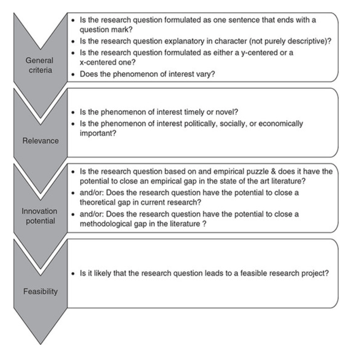
Checklist: Good research questions for social science projects (Panke, 2018)

Research Hypotheses

Present the researcher’s predictions based on specific statements.

• These statements define the research problem or issue and indicate the direction of the researcher’s predictions.
• Formulating the research question and hypothesis from existing data (e.g., a database) can lead to multiple statistical comparisons and potentially spurious findings due to chance.
• The research or clinical hypothesis, derived from the research question, shapes the study’s key elements: sampling strategy, intervention, comparison, and outcome variables.
• Hypotheses can express a single outcome or multiple outcomes.
• After statistical testing, the null hypothesis is either rejected or not rejected based on whether the study’s findings are statistically significant.
• Hypothesis testing helps determine if observed findings are due to true differences and not chance.
• Hypotheses can be 1-sided (specific direction of difference) or 2-sided (presence of a difference without specifying direction).
• 2-sided hypotheses are generally preferred unless there’s a strong justification for a 1-sided hypothesis.
• A solid research hypothesis, informed by a good research question, influences the research design and paves the way for defining clear research objectives.

Types of Research Hypothesis

• In a Y-centered research design, the focus is on the dependent variable (DV) which is specified in the research question. Theories are then used to identify independent variables (IV) and explain their causal relationship with the DV.
• Example: “An increase in teacher-led instructional time (IV) is likely to improve student reading comprehension scores (DV), because extensive guided practice under expert supervision enhances learning retention and skill mastery.”
• Hypothesis Explanation: The dependent variable (student reading comprehension scores) is the focus, and the hypothesis explores how changes in the independent variable (teacher-led instructional time) affect it.
• In X-centered research designs, the independent variable is specified in the research question. Theories are used to determine potential dependent variables and the causal mechanisms at play.
• Example: “Implementing technology-based learning tools (IV) is likely to enhance student engagement in the classroom (DV), because interactive and multimedia content increases student interest and participation.”
• Hypothesis Explanation: The independent variable (technology-based learning tools) is the focus, with the hypothesis exploring its impact on a potential dependent variable (student engagement).
• Probabilistic hypotheses suggest that changes in the independent variable are likely to lead to changes in the dependent variable in a predictable manner, but not with absolute certainty.
• Example: “The more teachers engage in professional development programs (IV), the more their teaching effectiveness (DV) is likely to improve, because continuous training updates pedagogical skills and knowledge.”
• Hypothesis Explanation: This hypothesis implies a probable relationship between the extent of professional development (IV) and teaching effectiveness (DV).
• Deterministic hypotheses state that a specific change in the independent variable will lead to a specific change in the dependent variable, implying a more direct and certain relationship.
• Example: “If the school curriculum changes from traditional lecture-based methods to project-based learning (IV), then student collaboration skills (DV) are expected to improve because project-based learning inherently requires teamwork and peer interaction.”
• Hypothesis Explanation: This hypothesis presumes a direct and definite outcome (improvement in collaboration skills) resulting from a specific change in the teaching method.
• Example : “Students who identify as visual learners will score higher on tests that are presented in a visually rich format compared to tests presented in a text-only format.”
• Explanation : This hypothesis aims to describe the potential difference in test scores between visual learners taking visually rich tests and text-only tests, without implying a direct cause-and-effect relationship.
• Example : “Teaching method A will improve student performance more than method B.”
• Explanation : This hypothesis compares the effectiveness of two different teaching methods, suggesting that one will lead to better student performance than the other. It implies a direct comparison but does not necessarily establish a causal mechanism.
• Example : “Students with higher self-efficacy will show higher levels of academic achievement.”
• Explanation : This hypothesis predicts a relationship between the variable of self-efficacy and academic achievement. Unlike a causal hypothesis, it does not necessarily suggest that one variable causes changes in the other, but rather that they are related in some way.

Tips for developing research questions and hypotheses for research studies

• Perform a systematic literature review (if one has not been done) to increase knowledge and familiarity with the topic and to assist with research development.
• Learn about current trends and technological advances on the topic.
• Seek careful input from experts, mentors, colleagues, and collaborators to refine your research question as this will aid in developing the research question and guide the research study.
• Use the FINER criteria in the development of the research question.
• Ensure that the research question follows PICOT format.
• Develop a research hypothesis from the research question.
• Ensure that the research question and objectives are answerable, feasible, and clinically relevant.

If your research hypotheses are derived from your research questions, particularly when multiple hypotheses address a single question, it’s recommended to use both research questions and hypotheses. However, if this isn’t the case, using hypotheses over research questions is advised. It’s important to note these are general guidelines, not strict rules. If you opt not to use hypotheses, consult with your supervisor for the best approach.

Farrugia, P., Petrisor, B. A., Farrokhyar, F., & Bhandari, M. (2010). Practical tips for surgical research: Research questions, hypotheses and objectives.  Canadian journal of surgery. Journal canadien de chirurgie ,  53 (4), 278–281.

Hulley, S. B., Cummings, S. R., Browner, W. S., Grady, D., & Newman, T. B. (2007). Designing clinical research. Philadelphia.

Panke, D. (2018). Research design & method selection: Making good choices in the social sciences.  Research Design & Method Selection , 1-368.

• Skip to secondary menu
• Skip to main content
• Skip to primary sidebar

Statistics By Jim

Making statistics intuitive

Null Hypothesis: Definition, Rejecting & Examples

By Jim Frost 6 Comments

What is a Null Hypothesis?

The null hypothesis in statistics states that there is no difference between groups or no relationship between variables. It is one of two mutually exclusive hypotheses about a population in a hypothesis test.

• Null Hypothesis H 0 : No effect exists in the population.
• Alternative Hypothesis H A : The effect exists in the population.

In every study or experiment, researchers assess an effect or relationship. This effect can be the effectiveness of a new drug, building material, or other intervention that has benefits. There is a benefit or connection that the researchers hope to identify. Unfortunately, no effect may exist. In statistics, we call this lack of an effect the null hypothesis. Researchers assume that this notion of no effect is correct until they have enough evidence to suggest otherwise, similar to how a trial presumes innocence.

In this context, the analysts don’t necessarily believe the null hypothesis is correct. In fact, they typically want to reject it because that leads to more exciting finds about an effect or relationship. The new vaccine works!

You can think of it as the default theory that requires sufficiently strong evidence to reject. Like a prosecutor, researchers must collect sufficient evidence to overturn the presumption of no effect. Investigators must work hard to set up a study and a data collection system to obtain evidence that can reject the null hypothesis.

Related post : What is an Effect in Statistics?

Null Hypothesis Examples

Null hypotheses start as research questions that the investigator rephrases as a statement indicating there is no effect or relationship.

After reading these examples, you might think they’re a bit boring and pointless. However, the key is to remember that the null hypothesis defines the condition that the researchers need to discredit before suggesting an effect exists.

Let’s see how you reject the null hypothesis and get to those more exciting findings!

When to Reject the Null Hypothesis

So, you want to reject the null hypothesis, but how and when can you do that? To start, you’ll need to perform a statistical test on your data. The following is an overview of performing a study that uses a hypothesis test.

The first step is to devise a research question and the appropriate null hypothesis. After that, the investigators need to formulate an experimental design and data collection procedures that will allow them to gather data that can answer the research question. Then they collect the data. For more information about designing a scientific study that uses statistics, read my post 5 Steps for Conducting Studies with Statistics .

After data collection is complete, statistics and hypothesis testing enter the picture. Hypothesis testing takes your sample data and evaluates how consistent they are with the null hypothesis. The p-value is a crucial part of the statistical results because it quantifies how strongly the sample data contradict the null hypothesis.

When the sample data provide sufficient evidence, you can reject the null hypothesis. In a hypothesis test, this process involves comparing the p-value to your significance level .

Rejecting the Null Hypothesis

Reject the null hypothesis when the p-value is less than or equal to your significance level. Your sample data favor the alternative hypothesis, which suggests that the effect exists in the population. For a mnemonic device, remember—when the p-value is low, the null must go!

When you can reject the null hypothesis, your results are statistically significant. Learn more about Statistical Significance: Definition & Meaning .

Failing to Reject the Null Hypothesis

Conversely, when the p-value is greater than your significance level, you fail to reject the null hypothesis. The sample data provides insufficient data to conclude that the effect exists in the population. When the p-value is high, the null must fly!

Note that failing to reject the null is not the same as proving it. For more information about the difference, read my post about Failing to Reject the Null .

That’s a very general look at the process. But I hope you can see how the path to more exciting findings depends on being able to rule out the less exciting null hypothesis that states there’s nothing to see here!

Let’s move on to learning how to write the null hypothesis for different types of effects, relationships, and tests.

Related posts : How Hypothesis Tests Work and Interpreting P-values

How to Write a Null Hypothesis

The null hypothesis varies by the type of statistic and hypothesis test. Remember that inferential statistics use samples to draw conclusions about populations. Consequently, when you write a null hypothesis, it must make a claim about the relevant population parameter . Further, that claim usually indicates that the effect does not exist in the population. Below are typical examples of writing a null hypothesis for various parameters and hypothesis tests.

Related posts : Descriptive vs. Inferential Statistics and Populations, Parameters, and Samples in Inferential Statistics

Group Means

T-tests and ANOVA assess the differences between group means. For these tests, the null hypothesis states that there is no difference between group means in the population. In other words, the experimental conditions that define the groups do not affect the mean outcome. Mu (µ) is the population parameter for the mean, and you’ll need to include it in the statement for this type of study.

For example, an experiment compares the mean bone density changes for a new osteoporosis medication. The control group does not receive the medicine, while the treatment group does. The null states that the mean bone density changes for the control and treatment groups are equal.

• Null Hypothesis H 0 : Group means are equal in the population: µ 1 = µ 2 , or µ 1 – µ 2 = 0
• Alternative Hypothesis H A : Group means are not equal in the population: µ 1 ≠ µ 2 , or µ 1 – µ 2 ≠ 0.

Group Proportions

Proportions tests assess the differences between group proportions. For these tests, the null hypothesis states that there is no difference between group proportions. Again, the experimental conditions did not affect the proportion of events in the groups. P is the population proportion parameter that you’ll need to include.

For example, a vaccine experiment compares the infection rate in the treatment group to the control group. The treatment group receives the vaccine, while the control group does not. The null states that the infection rates for the control and treatment groups are equal.

• Null Hypothesis H 0 : Group proportions are equal in the population: p 1 = p 2 .
• Alternative Hypothesis H A : Group proportions are not equal in the population: p 1 ≠ p 2 .

Correlation and Regression Coefficients

Some studies assess the relationship between two continuous variables rather than differences between groups.

In these studies, analysts often use either correlation or regression analysis . For these tests, the null states that there is no relationship between the variables. Specifically, it says that the correlation or regression coefficient is zero. As one variable increases, there is no tendency for the other variable to increase or decrease. Rho (ρ) is the population correlation parameter and beta (β) is the regression coefficient parameter.

For example, a study assesses the relationship between screen time and test performance. The null states that there is no correlation between this pair of variables. As screen time increases, test performance does not tend to increase or decrease.

• Null Hypothesis H 0 : The correlation in the population is zero: ρ = 0.
• Alternative Hypothesis H A : The correlation in the population is not zero: ρ ≠ 0.

For all these cases, the analysts define the hypotheses before the study. After collecting the data, they perform a hypothesis test to determine whether they can reject the null hypothesis.

The preceding examples are all for two-tailed hypothesis tests. To learn about one-tailed tests and how to write a null hypothesis for them, read my post One-Tailed vs. Two-Tailed Tests .

Related post : Understanding Correlation

Neyman, J; Pearson, E. S. (January 1, 1933).  On the Problem of the most Efficient Tests of Statistical Hypotheses .  Philosophical Transactions of the Royal Society A .  231  (694–706): 289–337.

Share this:

Reader Interactions

January 11, 2024 at 2:57 pm

Thanks for the reply.

January 10, 2024 at 1:23 pm

Hi Jim, In your comment you state that equivalence test null and alternate hypotheses are reversed. For hypothesis tests of data fits to a probability distribution, the null hypothesis is that the probability distribution fits the data. Is this correct?

January 10, 2024 at 2:15 pm

Those two separate things, equivalence testing and normality tests. But, yes, you’re correct for both.

Hypotheses are switched for equivalence testing. You need to “work” (i.e., collect a large sample of good quality data) to be able to reject the null that the groups are different to be able to conclude they’re the same.

With typical hypothesis tests, if you have low quality data and a low sample size, you’ll fail to reject the null that they’re the same, concluding they’re equivalent. But that’s more a statement about the low quality and small sample size than anything to do with the groups being equal.

So, equivalence testing make you work to obtain a finding that the groups are the same (at least within some amount you define as a trivial difference).

For normality testing, and other distribution tests, the null states that the data follow the distribution (normal or whatever). If you reject the null, you have sufficient evidence to conclude that your sample data don’t follow the probability distribution. That’s a rare case where you hope to fail to reject the null. And it suffers from the problem I describe above where you might fail to reject the null simply because you have a small sample size. In that case, you’d conclude the data follow the probability distribution but it’s more that you don’t have enough data for the test to register the deviation. In this scenario, if you had a larger sample size, you’d reject the null and conclude it doesn’t follow that distribution.

I don’t know of any equivalence testing type approach for distribution fit tests where you’d need to work to show the data follow a distribution, although I haven’t looked for one either!

February 20, 2022 at 9:26 pm

Is a null hypothesis regularly (always) stated in the negative? “there is no” or “does not”

February 23, 2022 at 9:21 pm

Typically, the null hypothesis includes an equal sign. The null hypothesis states that the population parameter equals a particular value. That value is usually one that represents no effect. In the case of a one-sided hypothesis test, the null still contains an equal sign but it’s “greater than or equal to” or “less than or equal to.” If you wanted to translate the null hypothesis from its native mathematical expression, you could use the expression “there is no effect.” But the mathematical form more specifically states what it’s testing.

It’s the alternative hypothesis that typically contains does not equal.

There are some exceptions. For example, in an equivalence test where the researchers want to show that two things are equal, the null hypothesis states that they’re not equal.

In short, the null hypothesis states the condition that the researchers hope to reject. They need to work hard to set up an experiment and data collection that’ll gather enough evidence to be able to reject the null condition.

February 15, 2022 at 9:32 am

Dear sir I always read your notes on Research methods.. Kindly tell is there any available Book on all these..wonderfull Urgent

Comments and Questions Cancel reply

• Privacy Policy

Home » Research Question Vs Hypothesis

Research Question Vs Hypothesis

Table of Contents

Research questions and hypotheses are both important elements of a research study, but they serve different purposes.

Research Question

A Research Question is a clear, concise, and specific question that a researcher asks to guide their study. Research questions are used to define the scope of the research project and to guide the collection and analysis of data. Research questions are often used in exploratory or descriptive studies, and they are open-ended in nature. Research questions should be answerable through data collection and analysis and should be linked to the research objectives or goals of the study.

A Hypothesis is a statement that predicts the relationship between two or more variables in a research study. Hypotheses are used in studies that aim to test cause-and-effect relationships between variables. A hypothesis is a tentative explanation for an observed phenomenon, and it is often derived from existing theory or previous research. Hypotheses are typically expressed as an “if-then” statement, where the “if” part refers to the independent variable, and the “then” part refers to the dependent variable. Hypotheses can be either directional (predicting the direction of the relationship between variables) or non-directional (predicting the presence of a relationship without specifying its direction).

Difference Between Research Question and Hypothesis

Here are some key differences between research questions and hypotheses:

Both Research Questions and Hypotheses are essential elements of a research study, but they serve different purposes. Research questions guide the study and help researchers define its scope, while hypotheses are used to test specific cause-and-effect relationships between variables. The choice of which to use depends on the nature of the research question, the study design, and the research objectives.

About the author

Muhammad Hassan

Researcher, Academic Writer, Web developer

You may also like

Descriptive vs Inferential Statistics – All Key...

Correlational Research Vs Experimental Research

Inductive Vs Deductive Research

Descriptive vs Experimental Research

Research Hypothesis Vs Null Hypothesis

Essay Vs Research Paper

Have a thesis expert improve your writing

Check your thesis for plagiarism in 10 minutes, generate your apa citations for free.

• Knowledge Base
• Null and Alternative Hypotheses | Definitions & Examples

Null and Alternative Hypotheses | Definitions & Examples

Published on 5 October 2022 by Shaun Turney . Revised on 6 December 2022.

The null and alternative hypotheses are two competing claims that researchers weigh evidence for and against using a statistical test :

• Null hypothesis (H 0 ): There’s no effect in the population .
• Alternative hypothesis (H A ): There’s an effect in the population.

The effect is usually the effect of the independent variable on the dependent variable .

Table of contents

Answering your research question with hypotheses, what is a null hypothesis, what is an alternative hypothesis, differences between null and alternative hypotheses, how to write null and alternative hypotheses, frequently asked questions about null and alternative hypotheses.

The null and alternative hypotheses offer competing answers to your research question . When the research question asks “Does the independent variable affect the dependent variable?”, the null hypothesis (H 0 ) answers “No, there’s no effect in the population.” On the other hand, the alternative hypothesis (H A ) answers “Yes, there is an effect in the population.”

The null and alternative are always claims about the population. That’s because the goal of hypothesis testing is to make inferences about a population based on a sample . Often, we infer whether there’s an effect in the population by looking at differences between groups or relationships between variables in the sample.

You can use a statistical test to decide whether the evidence favors the null or alternative hypothesis. Each type of statistical test comes with a specific way of phrasing the null and alternative hypothesis. However, the hypotheses can also be phrased in a general way that applies to any test.

The null hypothesis is the claim that there’s no effect in the population.

If the sample provides enough evidence against the claim that there’s no effect in the population ( p ≤ α), then we can reject the null hypothesis . Otherwise, we fail to reject the null hypothesis.

Although “fail to reject” may sound awkward, it’s the only wording that statisticians accept. Be careful not to say you “prove” or “accept” the null hypothesis.

Null hypotheses often include phrases such as “no effect”, “no difference”, or “no relationship”. When written in mathematical terms, they always include an equality (usually =, but sometimes ≥ or ≤).

Examples of null hypotheses

The table below gives examples of research questions and null hypotheses. There’s always more than one way to answer a research question, but these null hypotheses can help you get started.

*Note that some researchers prefer to always write the null hypothesis in terms of “no effect” and “=”. It would be fine to say that daily meditation has no effect on the incidence of depression and p 1 = p 2 .

The alternative hypothesis (H A ) is the other answer to your research question . It claims that there’s an effect in the population.

Often, your alternative hypothesis is the same as your research hypothesis. In other words, it’s the claim that you expect or hope will be true.

The alternative hypothesis is the complement to the null hypothesis. Null and alternative hypotheses are exhaustive, meaning that together they cover every possible outcome. They are also mutually exclusive, meaning that only one can be true at a time.

Alternative hypotheses often include phrases such as “an effect”, “a difference”, or “a relationship”. When alternative hypotheses are written in mathematical terms, they always include an inequality (usually ≠, but sometimes > or <). As with null hypotheses, there are many acceptable ways to phrase an alternative hypothesis.

Examples of alternative hypotheses

The table below gives examples of research questions and alternative hypotheses to help you get started with formulating your own.

Null and alternative hypotheses are similar in some ways:

• They’re both answers to the research question
• They both make claims about the population
• They’re both evaluated by statistical tests.

However, there are important differences between the two types of hypotheses, summarized in the following table.

To help you write your hypotheses, you can use the template sentences below. If you know which statistical test you’re going to use, you can use the test-specific template sentences. Otherwise, you can use the general template sentences.

The only thing you need to know to use these general template sentences are your dependent and independent variables. To write your research question, null hypothesis, and alternative hypothesis, fill in the following sentences with your variables:

Does independent variable affect dependent variable ?

• Null hypothesis (H 0 ): Independent variable does not affect dependent variable .
• Alternative hypothesis (H A ): Independent variable affects dependent variable .

Test-specific

Once you know the statistical test you’ll be using, you can write your hypotheses in a more precise and mathematical way specific to the test you chose. The table below provides template sentences for common statistical tests.

Note: The template sentences above assume that you’re performing one-tailed tests . One-tailed tests are appropriate for most studies.

The null hypothesis is often abbreviated as H 0 . When the null hypothesis is written using mathematical symbols, it always includes an equality symbol (usually =, but sometimes ≥ or ≤).

The alternative hypothesis is often abbreviated as H a or H 1 . When the alternative hypothesis is written using mathematical symbols, it always includes an inequality symbol (usually ≠, but sometimes < or >).

A research hypothesis is your proposed answer to your research question. The research hypothesis usually includes an explanation (‘ x affects y because …’).

A statistical hypothesis, on the other hand, is a mathematical statement about a population parameter. Statistical hypotheses always come in pairs: the null and alternative hypotheses. In a well-designed study , the statistical hypotheses correspond logically to the research hypothesis.

Cite this Scribbr article

If you want to cite this source, you can copy and paste the citation or click the ‘Cite this Scribbr article’ button to automatically add the citation to our free Reference Generator.

Turney, S. (2022, December 06). Null and Alternative Hypotheses | Definitions & Examples. Scribbr. Retrieved 16 September 2024, from https://www.scribbr.co.uk/stats/null-and-alternative-hypothesis/

Is this article helpful?

Shaun Turney

Other students also liked, levels of measurement: nominal, ordinal, interval, ratio, the standard normal distribution | calculator, examples & uses, types of variables in research | definitions & examples.

• Resources Home 🏠
• Try SciSpace Copilot
• Search research papers
• Add Copilot Extension
• Try AI Detector
• Try Paraphraser
• Try Citation Generator
• April Papers
• June Papers
• July Papers

The Craft of Writing a Strong Hypothesis

Table of Contents

Writing a hypothesis is one of the essential elements of a scientific research paper. It needs to be to the point, clearly communicating what your research is trying to accomplish. A blurry, drawn-out, or complexly-structured hypothesis can confuse your readers. Or worse, the editor and peer reviewers.

A captivating hypothesis is not too intricate. This blog will take you through the process so that, by the end of it, you have a better idea of how to convey your research paper's intent in just one sentence.

What is a Hypothesis?

The first step in your scientific endeavor, a hypothesis, is a strong, concise statement that forms the basis of your research. It is not the same as a thesis statement , which is a brief summary of your research paper .

The sole purpose of a hypothesis is to predict your paper's findings, data, and conclusion. It comes from a place of curiosity and intuition . When you write a hypothesis, you're essentially making an educated guess based on scientific prejudices and evidence, which is further proven or disproven through the scientific method.

The reason for undertaking research is to observe a specific phenomenon. A hypothesis, therefore, lays out what the said phenomenon is. And it does so through two variables, an independent and dependent variable.

The independent variable is the cause behind the observation, while the dependent variable is the effect of the cause. A good example of this is “mixing red and blue forms purple.” In this hypothesis, mixing red and blue is the independent variable as you're combining the two colors at your own will. The formation of purple is the dependent variable as, in this case, it is conditional to the independent variable.

Different Types of Hypotheses‌

Types of hypotheses

Some would stand by the notion that there are only two types of hypotheses: a Null hypothesis and an Alternative hypothesis. While that may have some truth to it, it would be better to fully distinguish the most common forms as these terms come up so often, which might leave you out of context.

Apart from Null and Alternative, there are Complex, Simple, Directional, Non-Directional, Statistical, and Associative and casual hypotheses. They don't necessarily have to be exclusive, as one hypothesis can tick many boxes, but knowing the distinctions between them will make it easier for you to construct your own.

1. Null hypothesis

A null hypothesis proposes no relationship between two variables. Denoted by H 0 , it is a negative statement like “Attending physiotherapy sessions does not affect athletes' on-field performance.” Here, the author claims physiotherapy sessions have no effect on on-field performances. Even if there is, it's only a coincidence.

2. Alternative hypothesis

Considered to be the opposite of a null hypothesis, an alternative hypothesis is donated as H1 or Ha. It explicitly states that the dependent variable affects the independent variable. A good  alternative hypothesis example is “Attending physiotherapy sessions improves athletes' on-field performance.” or “Water evaporates at 100 °C. ” The alternative hypothesis further branches into directional and non-directional.

• Directional hypothesis: A hypothesis that states the result would be either positive or negative is called directional hypothesis. It accompanies H1 with either the ‘<' or ‘>' sign.
• Non-directional hypothesis: A non-directional hypothesis only claims an effect on the dependent variable. It does not clarify whether the result would be positive or negative. The sign for a non-directional hypothesis is ‘≠.'

3. Simple hypothesis

A simple hypothesis is a statement made to reflect the relation between exactly two variables. One independent and one dependent. Consider the example, “Smoking is a prominent cause of lung cancer." The dependent variable, lung cancer, is dependent on the independent variable, smoking.

4. Complex hypothesis

In contrast to a simple hypothesis, a complex hypothesis implies the relationship between multiple independent and dependent variables. For instance, “Individuals who eat more fruits tend to have higher immunity, lesser cholesterol, and high metabolism.” The independent variable is eating more fruits, while the dependent variables are higher immunity, lesser cholesterol, and high metabolism.

5. Associative and casual hypothesis

Associative and casual hypotheses don't exhibit how many variables there will be. They define the relationship between the variables. In an associative hypothesis, changing any one variable, dependent or independent, affects others. In a casual hypothesis, the independent variable directly affects the dependent.

6. Empirical hypothesis

Also referred to as the working hypothesis, an empirical hypothesis claims a theory's validation via experiments and observation. This way, the statement appears justifiable and different from a wild guess.

Say, the hypothesis is “Women who take iron tablets face a lesser risk of anemia than those who take vitamin B12.” This is an example of an empirical hypothesis where the researcher  the statement after assessing a group of women who take iron tablets and charting the findings.

7. Statistical hypothesis

The point of a statistical hypothesis is to test an already existing hypothesis by studying a population sample. Hypothesis like “44% of the Indian population belong in the age group of 22-27.” leverage evidence to prove or disprove a particular statement.

Characteristics of a Good Hypothesis

Writing a hypothesis is essential as it can make or break your research for you. That includes your chances of getting published in a journal. So when you're designing one, keep an eye out for these pointers:

• A research hypothesis has to be simple yet clear to look justifiable enough.
• It has to be testable — your research would be rendered pointless if too far-fetched into reality or limited by technology.
• It has to be precise about the results —what you are trying to do and achieve through it should come out in your hypothesis.
• A research hypothesis should be self-explanatory, leaving no doubt in the reader's mind.
• If you are developing a relational hypothesis, you need to include the variables and establish an appropriate relationship among them.
• A hypothesis must keep and reflect the scope for further investigations and experiments.

Separating a Hypothesis from a Prediction

Outside of academia, hypothesis and prediction are often used interchangeably. In research writing, this is not only confusing but also incorrect. And although a hypothesis and prediction are guesses at their core, there are many differences between them.

A hypothesis is an educated guess or even a testable prediction validated through research. It aims to analyze the gathered evidence and facts to define a relationship between variables and put forth a logical explanation behind the nature of events.

Predictions are assumptions or expected outcomes made without any backing evidence. They are more fictionally inclined regardless of where they originate from.

For this reason, a hypothesis holds much more weight than a prediction. It sticks to the scientific method rather than pure guesswork. "Planets revolve around the Sun." is an example of a hypothesis as it is previous knowledge and observed trends. Additionally, we can test it through the scientific method.

Whereas "COVID-19 will be eradicated by 2030." is a prediction. Even though it results from past trends, we can't prove or disprove it. So, the only way this gets validated is to wait and watch if COVID-19 cases end by 2030.

Finally, How to Write a Hypothesis

Quick tips on writing a hypothesis

1.  Be clear about your research question

A hypothesis should instantly address the research question or the problem statement. To do so, you need to ask a question. Understand the constraints of your undertaken research topic and then formulate a simple and topic-centric problem. Only after that can you develop a hypothesis and further test for evidence.

2. Carry out a recce

Once you have your research's foundation laid out, it would be best to conduct preliminary research. Go through previous theories, academic papers, data, and experiments before you start curating your research hypothesis. It will give you an idea of your hypothesis's viability or originality.

Making use of references from relevant research papers helps draft a good research hypothesis. SciSpace Discover offers a repository of over 270 million research papers to browse through and gain a deeper understanding of related studies on a particular topic. Additionally, you can use SciSpace Copilot , your AI research assistant, for reading any lengthy research paper and getting a more summarized context of it. A hypothesis can be formed after evaluating many such summarized research papers. Copilot also offers explanations for theories and equations, explains paper in simplified version, allows you to highlight any text in the paper or clip math equations and tables and provides a deeper, clear understanding of what is being said. This can improve the hypothesis by helping you identify potential research gaps.

3. Create a 3-dimensional hypothesis

Variables are an essential part of any reasonable hypothesis. So, identify your independent and dependent variable(s) and form a correlation between them. The ideal way to do this is to write the hypothetical assumption in the ‘if-then' form. If you use this form, make sure that you state the predefined relationship between the variables.

In another way, you can choose to present your hypothesis as a comparison between two variables. Here, you must specify the difference you expect to observe in the results.

4. Write the first draft

Now that everything is in place, it's time to write your hypothesis. For starters, create the first draft. In this version, write what you expect to find from your research.

Clearly separate your independent and dependent variables and the link between them. Don't fixate on syntax at this stage. The goal is to ensure your hypothesis addresses the issue.

5. Proof your hypothesis

After preparing the first draft of your hypothesis, you need to inspect it thoroughly. It should tick all the boxes, like being concise, straightforward, relevant, and accurate. Your final hypothesis has to be well-structured as well.

Research projects are an exciting and crucial part of being a scholar. And once you have your research question, you need a great hypothesis to begin conducting research. Thus, knowing how to write a hypothesis is very important.

Now that you have a firmer grasp on what a good hypothesis constitutes, the different kinds there are, and what process to follow, you will find it much easier to write your hypothesis, which ultimately helps your research.

Now it's easier than ever to streamline your research workflow with SciSpace Discover . Its integrated, comprehensive end-to-end platform for research allows scholars to easily discover, write and publish their research and fosters collaboration.

It includes everything you need, including a repository of over 270 million research papers across disciplines, SEO-optimized summaries and public profiles to show your expertise and experience.

If you found these tips on writing a research hypothesis useful, head over to our blog on Statistical Hypothesis Testing to learn about the top researchers, papers, and institutions in this domain.

Frequently Asked Questions (FAQs)

1. what is the definition of hypothesis.

According to the Oxford dictionary, a hypothesis is defined as “An idea or explanation of something that is based on a few known facts, but that has not yet been proved to be true or correct”.

2. What is an example of hypothesis?

The hypothesis is a statement that proposes a relationship between two or more variables. An example: "If we increase the number of new users who join our platform by 25%, then we will see an increase in revenue."

3. What is an example of null hypothesis?

A null hypothesis is a statement that there is no relationship between two variables. The null hypothesis is written as H0. The null hypothesis states that there is no effect. For example, if you're studying whether or not a particular type of exercise increases strength, your null hypothesis will be "there is no difference in strength between people who exercise and people who don't."

4. What are the types of research?

• Fundamental research

• Applied research

• Qualitative research

• Quantitative research

• Mixed research

• Exploratory research

• Longitudinal research

• Cross-sectional research

• Field research

• Laboratory research

• Fixed research

• Flexible research

• Action research

• Policy research

• Classification research

• Comparative research

• Causal research

• Inductive research

• Deductive research

5. How to write a hypothesis?

• Your hypothesis should be able to predict the relationship and outcome.

• Avoid wordiness by keeping it simple and brief.

• Your hypothesis should contain observable and testable outcomes.

• Your hypothesis should be relevant to the research question.

6. What are the 2 types of hypothesis?

• Null hypotheses are used to test the claim that "there is no difference between two groups of data".

• Alternative hypotheses test the claim that "there is a difference between two data groups".

7. Difference between research question and research hypothesis?

A research question is a broad, open-ended question you will try to answer through your research. A hypothesis is a statement based on prior research or theory that you expect to be true due to your study. Example - Research question: What are the factors that influence the adoption of the new technology? Research hypothesis: There is a positive relationship between age, education and income level with the adoption of the new technology.

8. What is plural for hypothesis?

The plural of hypothesis is hypotheses. Here's an example of how it would be used in a statement, "Numerous well-considered hypotheses are presented in this part, and they are supported by tables and figures that are well-illustrated."

9. What is the red queen hypothesis?

The red queen hypothesis in evolutionary biology states that species must constantly evolve to avoid extinction because if they don't, they will be outcompeted by other species that are evolving. Leigh Van Valen first proposed it in 1973; since then, it has been tested and substantiated many times.

10. Who is known as the father of null hypothesis?

The father of the null hypothesis is Sir Ronald Fisher. He published a paper in 1925 that introduced the concept of null hypothesis testing, and he was also the first to use the term itself.

11. When to reject null hypothesis?

You need to find a significant difference between your two populations to reject the null hypothesis. You can determine that by running statistical tests such as an independent sample t-test or a dependent sample t-test. You should reject the null hypothesis if the p-value is less than 0.05.

You might also like

Consensus GPT vs. SciSpace GPT: Choose the Best GPT for Research

Literature Review and Theoretical Framework: Understanding the Differences

Types of Essays in Academic Writing - Quick Guide (2024)

User Preferences

Content preview.

Arcu felis bibendum ut tristique et egestas quis:

• Ut enim ad minim veniam, quis nostrud exercitation ullamco laboris
• Duis aute irure dolor in reprehenderit in voluptate
• Excepteur sint occaecat cupidatat non proident

Keyboard Shortcuts

10.1 - setting the hypotheses: examples.

A significance test examines whether the null hypothesis provides a plausible explanation of the data. The null hypothesis itself does not involve the data. It is a statement about a parameter (a numerical characteristic of the population). These population values might be proportions or means or differences between means or proportions or correlations or odds ratios or any other numerical summary of the population. The alternative hypothesis is typically the research hypothesis of interest. Here are some examples.

Example 10.2: Hypotheses with One Sample of One Categorical Variable Section  

About 10% of the human population is left-handed. Suppose a researcher at Penn State speculates that students in the College of Arts and Architecture are more likely to be left-handed than people found in the general population. We only have one sample since we will be comparing a population proportion based on a sample value to a known population value.

• Research Question : Are artists more likely to be left-handed than people found in the general population?
• Response Variable : Classification of the student as either right-handed or left-handed

State Null and Alternative Hypotheses

• Null Hypothesis : Students in the College of Arts and Architecture are no more likely to be left-handed than people in the general population (population percent of left-handed students in the College of Art and Architecture = 10% or p = .10).
• Alternative Hypothesis : Students in the College of Arts and Architecture are more likely to be left-handed than people in the general population (population percent of left-handed students in the College of Arts and Architecture > 10% or p > .10). This is a one-sided alternative hypothesis.

Example 10.3: Hypotheses with One Sample of One Measurement Variable Section  

A generic brand of the anti-histamine Diphenhydramine markets a capsule with a 50 milligram dose. The manufacturer is worried that the machine that fills the capsules has come out of calibration and is no longer creating capsules with the appropriate dosage.

• Research Question : Does the data suggest that the population mean dosage of this brand is different than 50 mg?
• Response Variable : dosage of the active ingredient found by a chemical assay.
• Null Hypothesis : On the average, the dosage sold under this brand is 50 mg (population mean dosage = 50 mg).
• Alternative Hypothesis : On the average, the dosage sold under this brand is not 50 mg (population mean dosage ≠ 50 mg). This is a two-sided alternative hypothesis.

Example 10.4: Hypotheses with Two Samples of One Categorical Variable Section  

Many people are starting to prefer vegetarian meals on a regular basis. Specifically, a researcher believes that females are more likely than males to eat vegetarian meals on a regular basis.

• Research Question : Does the data suggest that females are more likely than males to eat vegetarian meals on a regular basis?
• Response Variable : Classification of whether or not a person eats vegetarian meals on a regular basis
• Explanatory (Grouping) Variable: Sex
• Null Hypothesis : There is no sex effect regarding those who eat vegetarian meals on a regular basis (population percent of females who eat vegetarian meals on a regular basis = population percent of males who eat vegetarian meals on a regular basis or p females = p males ).
• Alternative Hypothesis : Females are more likely than males to eat vegetarian meals on a regular basis (population percent of females who eat vegetarian meals on a regular basis > population percent of males who eat vegetarian meals on a regular basis or p females > p males ). This is a one-sided alternative hypothesis.

Example 10.5: Hypotheses with Two Samples of One Measurement Variable Section  

Obesity is a major health problem today. Research is starting to show that people may be able to lose more weight on a low carbohydrate diet than on a low fat diet.

• Research Question : Does the data suggest that, on the average, people are able to lose more weight on a low carbohydrate diet than on a low fat diet?
• Response Variable : Weight loss (pounds)
• Explanatory (Grouping) Variable : Type of diet
• Null Hypothesis : There is no difference in the mean amount of weight loss when comparing a low carbohydrate diet with a low fat diet (population mean weight loss on a low carbohydrate diet = population mean weight loss on a low fat diet).
• Alternative Hypothesis : The mean weight loss should be greater for those on a low carbohydrate diet when compared with those on a low fat diet (population mean weight loss on a low carbohydrate diet > population mean weight loss on a low fat diet). This is a one-sided alternative hypothesis.

Example 10.6: Hypotheses about the relationship between Two Categorical Variables Section  

• Research Question : Do the odds of having a stroke increase if you inhale second hand smoke ? A case-control study of non-smoking stroke patients and controls of the same age and occupation are asked if someone in their household smokes.
• Variables : There are two different categorical variables (Stroke patient vs control and whether the subject lives in the same household as a smoker). Living with a smoker (or not) is the natural explanatory variable and having a stroke (or not) is the natural response variable in this situation.
• Null Hypothesis : There is no relationship between whether or not a person has a stroke and whether or not a person lives with a smoker (odds ratio between stroke and second-hand smoke situation is = 1).
• Alternative Hypothesis : There is a relationship between whether or not a person has a stroke and whether or not a person lives with a smoker (odds ratio between stroke and second-hand smoke situation is > 1). This is a one-tailed alternative.

This research question might also be addressed like example 11.4 by making the hypotheses about comparing the proportion of stroke patients that live with smokers to the proportion of controls that live with smokers.

Example 10.7: Hypotheses about the relationship between Two Measurement Variables Section  

• Research Question : A financial analyst believes there might be a positive association between the change in a stock's price and the amount of the stock purchased by non-management employees the previous day (stock trading by management being under "insider-trading" regulatory restrictions).
• Variables : Daily price change information (the response variable) and previous day stock purchases by non-management employees (explanatory variable). These are two different measurement variables.
• Null Hypothesis : The correlation between the daily stock price change (\$) and the daily stock purchases by non-management employees (\$) = 0.
• Alternative Hypothesis : The correlation between the daily stock price change (\$) and the daily stock purchases by non-management employees (\$) > 0. This is a one-sided alternative hypothesis.

Example 10.8: Hypotheses about comparing the relationship between Two Measurement Variables in Two Samples Section  

• Research Question : Is there a linear relationship between the amount of the bill (\$) at a restaurant and the tip (\$) that was left. Is the strength of this association different for family restaurants than for fine dining restaurants?
• Variables : There are two different measurement variables. The size of the tip would depend on the size of the bill so the amount of the bill would be the explanatory variable and the size of the tip would be the response variable.
• Null Hypothesis : The correlation between the amount of the bill (\$) at a restaurant and the tip (\$) that was left is the same at family restaurants as it is at fine dining restaurants.
• Alternative Hypothesis : The correlation between the amount of the bill (\$) at a restaurant and the tip (\$) that was left is the difference at family restaurants then it is at fine dining restaurants. This is a two-sided alternative hypothesis.

Statistics Resources

• Excel - Tutorials
• Basic Probability Rules
• Single Event Probability
• Complement Rule
• Intersections & Unions
• Compound Events
• Levels of Measurement
• Independent and Dependent Variables
• Entering Data
• Central Tendency
• Data and Tests
• Displaying Data
• Discussing Statistics In-text
• SEM and Confidence Intervals
• Two-Way Frequency Tables
• Empirical Rule
• Finding Probability
• Accessing SPSS
• Chart and Graphs
• Frequency Table and Distribution
• Descriptive Statistics
• Converting Raw Scores to Z-Scores
• Converting Z-scores to t-scores
• Split File/Split Output
• Partial Eta Squared
• Downloading and Installing G*Power: Windows/PC
• Correlation
• Testing Parametric Assumptions
• One-Way ANOVA
• Two-Way ANOVA
• Repeated Measures ANOVA
• Goodness-of-Fit
• Test of Association
• Pearson's r
• Point Biserial
• Mediation and Moderation
• Simple Linear Regression
• Multiple Linear Regression
• Binomial Logistic Regression
• Multinomial Logistic Regression
• Independent Samples T-test
• Dependent Samples T-test
• Testing Assumptions
• T-tests using SPSS
• T-Test Practice
• Predictive Analytics This link opens in a new window
• Quantitative Research Questions
• Null & Alternative Hypotheses
• One-Tail vs. Two-Tail
• Alpha & Beta
• Associated Probability
• Decision Rule
• Statement of Conclusion
• Statistics Group Sessions

ASC Chat Hours

ASC Chat is usually available at the following times ( Pacific Time):

If there is not a coach on duty, submit your question via one of the below methods:

  928-440-1325

  Ask a Coach

  [email protected]

Search our FAQs on the Academic Success Center's  Ask a Coach   page.

Once you have developed a clear and focused research question or set of research questions, you’ll be ready to conduct further research, a literature review, on the topic to help you make an educated guess about the answer to your question(s). This educated guess is called a hypothesis.

In research, there are two types of hypotheses: null and alternative. They work as a complementary pair, each stating that the other is wrong.

• Null Hypothesis (H 0 ) – This can be thought of as the implied hypothesis. “Null” meaning “nothing.”  This hypothesis states that there is no difference between groups or no relationship between variables. The null hypothesis is a presumption of status quo or no change.
• Alternative Hypothesis (H a ) – This is also known as the claim. This hypothesis should state what you expect the data to show, based on your research on the topic. This is your answer to your research question.

Null Hypothesis:   H 0 : There is no difference in the salary of factory workers based on gender. Alternative Hypothesis :  H a : Male factory workers have a higher salary than female factory workers.

Null Hypothesis :  H 0 : There is no relationship between height and shoe size. Alternative Hypothesis :  H a : There is a positive relationship between height and shoe size.

Null Hypothesis :  H 0 : Experience on the job has no impact on the quality of a brick mason’s work. Alternative Hypothesis :  H a : The quality of a brick mason’s work is influenced by on-the-job experience.

Was this resource helpful?

• << Previous: Hypothesis Testing
• Next: One-Tail vs. Two-Tail >>
• Last Updated: Jul 16, 2024 11:19 AM
• URL: https://resources.nu.edu/statsresources

What is The Null Hypothesis & When Do You Reject The Null Hypothesis

Julia Simkus

Editor at Simply Psychology

BA (Hons) Psychology, Princeton University

Julia Simkus is a graduate of Princeton University with a Bachelor of Arts in Psychology. She is currently studying for a Master's Degree in Counseling for Mental Health and Wellness in September 2023. Julia's research has been published in peer reviewed journals.

Learn about our Editorial Process

Saul McLeod, PhD

Editor-in-Chief for Simply Psychology

BSc (Hons) Psychology, MRes, PhD, University of Manchester

Saul McLeod, PhD., is a qualified psychology teacher with over 18 years of experience in further and higher education. He has been published in peer-reviewed journals, including the Journal of Clinical Psychology.

Olivia Guy-Evans, MSc

Associate Editor for Simply Psychology

BSc (Hons) Psychology, MSc Psychology of Education

Olivia Guy-Evans is a writer and associate editor for Simply Psychology. She has previously worked in healthcare and educational sectors.

On This Page:

A null hypothesis is a statistical concept suggesting no significant difference or relationship between measured variables. It’s the default assumption unless empirical evidence proves otherwise.

The null hypothesis states no relationship exists between the two variables being studied (i.e., one variable does not affect the other).

The null hypothesis is the statement that a researcher or an investigator wants to disprove.

Testing the null hypothesis can tell you whether your results are due to the effects of manipulating ​ the dependent variable or due to random chance. 

How to Write a Null Hypothesis

Null hypotheses (H0) start as research questions that the investigator rephrases as statements indicating no effect or relationship between the independent and dependent variables.

It is a default position that your research aims to challenge or confirm.

For example, if studying the impact of exercise on weight loss, your null hypothesis might be:

There is no significant difference in weight loss between individuals who exercise daily and those who do not.

Examples of Null Hypotheses

When Do We Reject The Null Hypothesis? 

We reject the null hypothesis when the data provide strong enough evidence to conclude that it is likely incorrect. This often occurs when the p-value (probability of observing the data given the null hypothesis is true) is below a predetermined significance level.

If the collected data does not meet the expectation of the null hypothesis, a researcher can conclude that the data lacks sufficient evidence to back up the null hypothesis, and thus the null hypothesis is rejected. 

Rejecting the null hypothesis means that a relationship does exist between a set of variables and the effect is statistically significant ( p > 0.05).

If the data collected from the random sample is not statistically significance , then the null hypothesis will be accepted, and the researchers can conclude that there is no relationship between the variables. 

You need to perform a statistical test on your data in order to evaluate how consistent it is with the null hypothesis. A p-value is one statistical measurement used to validate a hypothesis against observed data.

Calculating the p-value is a critical part of null-hypothesis significance testing because it quantifies how strongly the sample data contradicts the null hypothesis.

The level of statistical significance is often expressed as a  p  -value between 0 and 1. The smaller the p-value, the stronger the evidence that you should reject the null hypothesis.

Usually, a researcher uses a confidence level of 95% or 99% (p-value of 0.05 or 0.01) as general guidelines to decide if you should reject or keep the null.

When your p-value is less than or equal to your significance level, you reject the null hypothesis.

In other words, smaller p-values are taken as stronger evidence against the null hypothesis. Conversely, when the p-value is greater than your significance level, you fail to reject the null hypothesis.

In this case, the sample data provides insufficient data to conclude that the effect exists in the population.

Because you can never know with complete certainty whether there is an effect in the population, your inferences about a population will sometimes be incorrect.

When you incorrectly reject the null hypothesis, it’s called a type I error. When you incorrectly fail to reject it, it’s called a type II error.

Why Do We Never Accept The Null Hypothesis?

The reason we do not say “accept the null” is because we are always assuming the null hypothesis is true and then conducting a study to see if there is evidence against it. And, even if we don’t find evidence against it, a null hypothesis is not accepted.

A lack of evidence only means that you haven’t proven that something exists. It does not prove that something doesn’t exist. 

It is risky to conclude that the null hypothesis is true merely because we did not find evidence to reject it. It is always possible that researchers elsewhere have disproved the null hypothesis, so we cannot accept it as true, but instead, we state that we failed to reject the null. 

One can either reject the null hypothesis, or fail to reject it, but can never accept it.

Why Do We Use The Null Hypothesis?

We can never prove with 100% certainty that a hypothesis is true; We can only collect evidence that supports a theory. However, testing a hypothesis can set the stage for rejecting or accepting this hypothesis within a certain confidence level.

The null hypothesis is useful because it can tell us whether the results of our study are due to random chance or the manipulation of a variable (with a certain level of confidence).

A null hypothesis is rejected if the measured data is significantly unlikely to have occurred and a null hypothesis is accepted if the observed outcome is consistent with the position held by the null hypothesis.

Rejecting the null hypothesis sets the stage for further experimentation to see if a relationship between two variables exists. 

Hypothesis testing is a critical part of the scientific method as it helps decide whether the results of a research study support a particular theory about a given population. Hypothesis testing is a systematic way of backing up researchers’ predictions with statistical analysis.

It helps provide sufficient statistical evidence that either favors or rejects a certain hypothesis about the population parameter. 

Purpose of a Null Hypothesis 

• The primary purpose of the null hypothesis is to disprove an assumption. 
• Whether rejected or accepted, the null hypothesis can help further progress a theory in many scientific cases.
• A null hypothesis can be used to ascertain how consistent the outcomes of multiple studies are.

Do you always need both a Null Hypothesis and an Alternative Hypothesis?

The null (H0) and alternative (Ha or H1) hypotheses are two competing claims that describe the effect of the independent variable on the dependent variable. They are mutually exclusive, which means that only one of the two hypotheses can be true. 

While the null hypothesis states that there is no effect in the population, an alternative hypothesis states that there is statistical significance between two variables. 

The goal of hypothesis testing is to make inferences about a population based on a sample. In order to undertake hypothesis testing, you must express your research hypothesis as a null and alternative hypothesis. Both hypotheses are required to cover every possible outcome of the study. 

What is the difference between a null hypothesis and an alternative hypothesis?

The alternative hypothesis is the complement to the null hypothesis. The null hypothesis states that there is no effect or no relationship between variables, while the alternative hypothesis claims that there is an effect or relationship in the population.

It is the claim that you expect or hope will be true. The null hypothesis and the alternative hypothesis are always mutually exclusive, meaning that only one can be true at a time.

What are some problems with the null hypothesis?

One major problem with the null hypothesis is that researchers typically will assume that accepting the null is a failure of the experiment. However, accepting or rejecting any hypothesis is a positive result. Even if the null is not refuted, the researchers will still learn something new.

Why can a null hypothesis not be accepted?

We can either reject or fail to reject a null hypothesis, but never accept it. If your test fails to detect an effect, this is not proof that the effect doesn’t exist. It just means that your sample did not have enough evidence to conclude that it exists.

We can’t accept a null hypothesis because a lack of evidence does not prove something that does not exist. Instead, we fail to reject it.

Failing to reject the null indicates that the sample did not provide sufficient enough evidence to conclude that an effect exists.

If the p-value is greater than the significance level, then you fail to reject the null hypothesis.

Is a null hypothesis directional or non-directional?

A hypothesis test can either contain an alternative directional hypothesis or a non-directional alternative hypothesis. A directional hypothesis is one that contains the less than (“<“) or greater than (“>”) sign.

A nondirectional hypothesis contains the not equal sign (“≠”).  However, a null hypothesis is neither directional nor non-directional.

A null hypothesis is a prediction that there will be no change, relationship, or difference between two variables.

The directional hypothesis or nondirectional hypothesis would then be considered alternative hypotheses to the null hypothesis.

Gill, J. (1999). The insignificance of null hypothesis significance testing.  Political research quarterly ,  52 (3), 647-674.

Krueger, J. (2001). Null hypothesis significance testing: On the survival of a flawed method.  American Psychologist ,  56 (1), 16.

Masson, M. E. (2011). A tutorial on a practical Bayesian alternative to null-hypothesis significance testing.  Behavior research methods ,  43 , 679-690.

Nickerson, R. S. (2000). Null hypothesis significance testing: a review of an old and continuing controversy.  Psychological methods ,  5 (2), 241.

Rozeboom, W. W. (1960). The fallacy of the null-hypothesis significance test.  Psychological bulletin ,  57 (5), 416.

Module 9: Hypothesis Testing With One Sample

Null and alternative hypotheses, learning outcomes.

• Describe hypothesis testing in general and in practice

The actual test begins by considering two  hypotheses . They are called the null hypothesis and the alternative hypothesis . These hypotheses contain opposing viewpoints.

H 0 : The null hypothesis: It is a statement about the population that either is believed to be true or is used to put forth an argument unless it can be shown to be incorrect beyond a reasonable doubt.

H a : The alternative hypothesis : It is a claim about the population that is contradictory to H 0 and what we conclude when we reject H 0 .

Since the null and alternative hypotheses are contradictory, you must examine evidence to decide if you have enough evidence to reject the null hypothesis or not. The evidence is in the form of sample data.

After you have determined which hypothesis the sample supports, you make adecision. There are two options for a  decision . They are “reject H 0 ” if the sample information favors the alternative hypothesis or “do not reject H 0 ” or “decline to reject H 0 ” if the sample information is insufficient to reject the null hypothesis.

Mathematical Symbols Used in  H 0 and H a :

H 0 always has a symbol with an equal in it. H a never has a symbol with an equal in it. The choice of symbol depends on the wording of the hypothesis test. However, be aware that many researchers (including one of the co-authors in research work) use = in the null hypothesis, even with > or < as the symbol in the alternative hypothesis. This practice is acceptable because we only make the decision to reject or not reject the null hypothesis.

H 0 : No more than 30% of the registered voters in Santa Clara County voted in the primary election. p ≤ 30

H a : More than 30% of the registered voters in Santa Clara County voted in the primary election. p > 30

A medical trial is conducted to test whether or not a new medicine reduces cholesterol by 25%. State the null and alternative hypotheses.

H 0 : The drug reduces cholesterol by 25%. p = 0.25

H a : The drug does not reduce cholesterol by 25%. p ≠ 0.25

We want to test whether the mean GPA of students in American colleges is different from 2.0 (out of 4.0). The null and alternative hypotheses are:

H 0 : μ = 2.0

H a : μ ≠ 2.0

We want to test whether the mean height of eighth graders is 66 inches. State the null and alternative hypotheses. Fill in the correct symbol (=, ≠, ≥, <, ≤, >) for the null and alternative hypotheses. H 0 : μ __ 66 H a : μ __ 66

• H 0 : μ = 66
• H a : μ ≠ 66

We want to test if college students take less than five years to graduate from college, on the average. The null and alternative hypotheses are:

H 0 : μ ≥ 5

H a : μ < 5

We want to test if it takes fewer than 45 minutes to teach a lesson plan. State the null and alternative hypotheses. Fill in the correct symbol ( =, ≠, ≥, <, ≤, >) for the null and alternative hypotheses. H 0 : μ __ 45 H a : μ __ 45

• H 0 : μ ≥ 45
• H a : μ < 45

In an issue of U.S. News and World Report , an article on school standards stated that about half of all students in France, Germany, and Israel take advanced placement exams and a third pass. The same article stated that 6.6% of U.S. students take advanced placement exams and 4.4% pass. Test if the percentage of U.S. students who take advanced placement exams is more than 6.6%. State the null and alternative hypotheses.

H 0 : p ≤ 0.066

H a : p > 0.066

On a state driver’s test, about 40% pass the test on the first try. We want to test if more than 40% pass on the first try. Fill in the correct symbol (=, ≠, ≥, <, ≤, >) for the null and alternative hypotheses. H 0 : p __ 0.40 H a : p __ 0.40

• H 0 : p = 0.40
• H a : p > 0.40

Concept Review

In a  hypothesis test , sample data is evaluated in order to arrive at a decision about some type of claim. If certain conditions about the sample are satisfied, then the claim can be evaluated for a population. In a hypothesis test, we: Evaluate the null hypothesis , typically denoted with H 0 . The null is not rejected unless the hypothesis test shows otherwise. The null statement must always contain some form of equality (=, ≤ or ≥) Always write the alternative hypothesis , typically denoted with H a or H 1 , using less than, greater than, or not equals symbols, i.e., (≠, >, or <). If we reject the null hypothesis, then we can assume there is enough evidence to support the alternative hypothesis. Never state that a claim is proven true or false. Keep in mind the underlying fact that hypothesis testing is based on probability laws; therefore, we can talk only in terms of non-absolute certainties.

Formula Review

H 0 and H a are contradictory.

• OpenStax, Statistics, Null and Alternative Hypotheses. Provided by : OpenStax. Located at : http://cnx.org/contents/[email protected]:58/Introductory_Statistics . License : CC BY: Attribution
• Introductory Statistics . Authored by : Barbara Illowski, Susan Dean. Provided by : Open Stax. Located at : http://cnx.org/contents/[email protected] . License : CC BY: Attribution . License Terms : Download for free at http://cnx.org/contents/[email protected]
• Simple hypothesis testing | Probability and Statistics | Khan Academy. Authored by : Khan Academy. Located at : https://youtu.be/5D1gV37bKXY . License : All Rights Reserved . License Terms : Standard YouTube License

• Key Differences

Know the Differences & Comparisons

Difference Between Null and Alternative Hypothesis

Null hypothesis implies a statement that expects no difference or effect. On the contrary, an alternative hypothesis is one that expects some difference or effect. Null hypothesis This article excerpt shed light on the fundamental differences between null and alternative hypothesis.

Content: Null Hypothesis Vs Alternative Hypothesis

Comparison chart.

Definition of Null Hypothesis

A null hypothesis is a statistical hypothesis in which there is no significant difference exist between the set of variables. It is the original or default statement, with no effect, often represented by H 0 (H-zero). It is always the hypothesis that is tested. It denotes the certain value of population parameter such as µ, s, p. A null hypothesis can be rejected, but it cannot be accepted just on the basis of a single test.

Definition of Alternative Hypothesis

A statistical hypothesis used in hypothesis testing, which states that there is a significant difference between the set of variables. It is often referred to as the hypothesis other than the null hypothesis, often denoted by H 1 (H-one). It is what the researcher seeks to prove in an indirect way, by using the test. It refers to a certain value of sample statistic, e.g., x¯, s, p

The acceptance of alternative hypothesis depends on the rejection of the null hypothesis i.e. until and unless null hypothesis is rejected, an alternative hypothesis cannot be accepted.

Key Differences Between Null and Alternative Hypothesis

The important points of differences between null and alternative hypothesis are explained as under:

• A null hypothesis is a statement, in which there is no relationship between two variables. An alternative hypothesis is a statement; that is simply the inverse of the null hypothesis, i.e. there is some statistical significance between two measured phenomenon.
• A null hypothesis is what, the researcher tries to disprove whereas an alternative hypothesis is what the researcher wants to prove.
• A null hypothesis represents, no observed effect whereas an alternative hypothesis reflects, some observed effect.
• If the null hypothesis is accepted, no changes will be made in the opinions or actions. Conversely, if the alternative hypothesis is accepted, it will result in the changes in the opinions or actions.
• As null hypothesis refers to population parameter, the testing is indirect and implicit. On the other hand, the alternative hypothesis indicates sample statistic, wherein, the testing is direct and explicit.
• A null hypothesis is labelled as H 0 (H-zero) while an alternative hypothesis is represented by H 1 (H-one).
• The mathematical formulation of a null hypothesis is an equal sign but for an alternative hypothesis is not equal to sign.
• In null hypothesis, the observations are the outcome of chance whereas, in the case of the alternative hypothesis, the observations are an outcome of real effect.

There are two outcomes of a statistical test, i.e. first, a null hypothesis is rejected and alternative hypothesis is accepted, second, null hypothesis is accepted, on the basis of the evidence. In simple terms, a null hypothesis is just opposite of alternative hypothesis.

You Might Also Like:

Zipporah Thuo says

February 22, 2018 at 6:06 pm

The comparisons between the two hypothesis i.e Null hypothesis and the Alternative hypothesis are the best.Thank you.

Getu Gamo says

March 4, 2019 at 3:42 am

Thank you so much for the detail explanation on two hypotheses. Now I understood both very well, including their differences.

Jyoti Bhardwaj says

May 28, 2019 at 6:26 am

Thanks, Surbhi! Appreciate the clarity and precision of this content.

January 9, 2020 at 6:16 am

John Jenstad says

July 20, 2020 at 2:52 am

Thanks very much, Surbhi, for your clear explanation!!

Navita says

July 2, 2021 at 11:48 am

Thanks for the Comparison chart! it clears much of my doubt.

GURU UPPALA says

July 21, 2022 at 8:36 pm

Thanks for the Comparison chart!

Enock kipkoech says

September 22, 2022 at 1:57 pm

What are the examples of null hypothesis and substantive hypothesis

Leave a Reply Cancel reply

Your email address will not be published. Required fields are marked *

Save my name, email, and website in this browser for the next time I comment.

Null Hypothesis Examples

ThoughtCo / Hilary Allison

• Scientific Method
• Chemical Laws
• Periodic Table
• Projects & Experiments
• Biochemistry
• Physical Chemistry
• Medical Chemistry
• Chemistry In Everyday Life
• Famous Chemists
• Activities for Kids
• Abbreviations & Acronyms
• Weather & Climate
• Ph.D., Biomedical Sciences, University of Tennessee at Knoxville
• B.A., Physics and Mathematics, Hastings College

In statistical analysis, the null hypothesis assumes there is no meaningful relationship between two variables. Testing the null hypothesis can tell you whether your results are due to the effect of manipulating ​a dependent variable or due to chance. It's often used in conjunction with an alternative hypothesis, which assumes there is, in fact, a relationship between two variables.

The null hypothesis is among the easiest hypothesis to test using statistical analysis, making it perhaps the most valuable hypothesis for the scientific method. By evaluating a null hypothesis in addition to another hypothesis, researchers can support their conclusions with a higher level of confidence. Below are examples of how you might formulate a null hypothesis to fit certain questions.

What Is the Null Hypothesis?

The null hypothesis states there is no relationship between the measured phenomenon (the dependent variable ) and the independent variable , which is the variable an experimenter typically controls or changes. You do not​ need to believe that the null hypothesis is true to test it. On the contrary, you will likely suspect there is a relationship between a set of variables. One way to prove that this is the case is to reject the null hypothesis. Rejecting a hypothesis does not mean an experiment was "bad" or that it didn't produce results. In fact, it is often one of the first steps toward further inquiry.

To distinguish it from other hypotheses , the null hypothesis is written as ​ H 0  (which is read as “H-nought,” "H-null," or "H-zero"). A significance test is used to determine the likelihood that the results supporting the null hypothesis are not due to chance. A confidence level of 95% or 99% is common. Keep in mind, even if the confidence level is high, there is still a small chance the null hypothesis is not true, perhaps because the experimenter did not account for a critical factor or because of chance. This is one reason why it's important to repeat experiments.

Examples of the Null Hypothesis

To write a null hypothesis, first start by asking a question. Rephrase that question in a form that assumes no relationship between the variables. In other words, assume a treatment has no effect. Write your hypothesis in a way that reflects this.

Other Types of Hypotheses

In addition to the null hypothesis, the alternative hypothesis is also a staple in traditional significance tests . It's essentially the opposite of the null hypothesis because it assumes the claim in question is true. For the first item in the table above, for example, an alternative hypothesis might be "Age does have an effect on mathematical ability."

Key Takeaways

• In hypothesis testing, the null hypothesis assumes no relationship between two variables, providing a baseline for statistical analysis.
• Rejecting the null hypothesis suggests there is evidence of a relationship between variables.
• By formulating a null hypothesis, researchers can systematically test assumptions and draw more reliable conclusions from their experiments.
• What Are Examples of a Hypothesis?
• Random Error vs. Systematic Error
• Six Steps of the Scientific Method
• What Is a Hypothesis? (Science)
• Scientific Method Flow Chart
• What Are the Elements of a Good Hypothesis?
• Scientific Method Vocabulary Terms
• Understanding Simple vs Controlled Experiments
• The Role of a Controlled Variable in an Experiment
• What Is an Experimental Constant?
• What Is a Testable Hypothesis?
• Scientific Hypothesis Examples
• What Is the Difference Between a Control Variable and Control Group?
• DRY MIX Experiment Variables Acronym
• What Is a Controlled Experiment?
• Scientific Variable

Frequently asked questions

What are null and alternative hypotheses.

Null and alternative hypotheses are used in statistical hypothesis testing . The null hypothesis of a test always predicts no effect or no relationship between variables, while the alternative hypothesis states your research prediction of an effect or relationship.

Frequently asked questions: Statistics

As the degrees of freedom increase, Student’s t distribution becomes less leptokurtic , meaning that the probability of extreme values decreases. The distribution becomes more and more similar to a standard normal distribution .

The three categories of kurtosis are:

• Mesokurtosis : An excess kurtosis of 0. Normal distributions are mesokurtic.
• Platykurtosis : A negative excess kurtosis. Platykurtic distributions are thin-tailed, meaning that they have few outliers .
• Leptokurtosis : A positive excess kurtosis. Leptokurtic distributions are fat-tailed, meaning that they have many outliers.

Probability distributions belong to two broad categories: discrete probability distributions and continuous probability distributions . Within each category, there are many types of probability distributions.

Probability is the relative frequency over an infinite number of trials.

For example, the probability of a coin landing on heads is .5, meaning that if you flip the coin an infinite number of times, it will land on heads half the time.

Since doing something an infinite number of times is impossible, relative frequency is often used as an estimate of probability. If you flip a coin 1000 times and get 507 heads, the relative frequency, .507, is a good estimate of the probability.

Categorical variables can be described by a frequency distribution. Quantitative variables can also be described by a frequency distribution, but first they need to be grouped into interval classes .

A histogram is an effective way to tell if a frequency distribution appears to have a normal distribution .

Plot a histogram and look at the shape of the bars. If the bars roughly follow a symmetrical bell or hill shape, like the example below, then the distribution is approximately normally distributed.

You can use the CHISQ.INV.RT() function to find a chi-square critical value in Excel.

For example, to calculate the chi-square critical value for a test with df = 22 and α = .05, click any blank cell and type:

=CHISQ.INV.RT(0.05,22)

You can use the qchisq() function to find a chi-square critical value in R.

For example, to calculate the chi-square critical value for a test with df = 22 and α = .05:

qchisq(p = .05, df = 22, lower.tail = FALSE)

You can use the chisq.test() function to perform a chi-square test of independence in R. Give the contingency table as a matrix for the “x” argument. For example:

m = matrix(data = c(89, 84, 86, 9, 8, 24), nrow = 3, ncol = 2)

chisq.test(x = m)

You can use the CHISQ.TEST() function to perform a chi-square test of independence in Excel. It takes two arguments, CHISQ.TEST(observed_range, expected_range), and returns the p value.

Chi-square goodness of fit tests are often used in genetics. One common application is to check if two genes are linked (i.e., if the assortment is independent). When genes are linked, the allele inherited for one gene affects the allele inherited for another gene.

Suppose that you want to know if the genes for pea texture (R = round, r = wrinkled) and color (Y = yellow, y = green) are linked. You perform a dihybrid cross between two heterozygous ( RY / ry ) pea plants. The hypotheses you’re testing with your experiment are:

• This would suggest that the genes are unlinked.
• This would suggest that the genes are linked.

You observe 100 peas:

• 78 round and yellow peas
• 6 round and green peas
• 4 wrinkled and yellow peas
• 12 wrinkled and green peas

Step 1: Calculate the expected frequencies

To calculate the expected values, you can make a Punnett square. If the two genes are unlinked, the probability of each genotypic combination is equal.

The expected phenotypic ratios are therefore 9 round and yellow: 3 round and green: 3 wrinkled and yellow: 1 wrinkled and green.

From this, you can calculate the expected phenotypic frequencies for 100 peas:

Step 2: Calculate chi-square

Χ 2 = 8.41 + 8.67 + 11.6 + 5.4 = 34.08

Step 3: Find the critical chi-square value

Since there are four groups (round and yellow, round and green, wrinkled and yellow, wrinkled and green), there are three degrees of freedom .

For a test of significance at α = .05 and df = 3, the Χ 2 critical value is 7.82.

Step 4: Compare the chi-square value to the critical value

Χ 2 = 34.08

Critical value = 7.82

The Χ 2 value is greater than the critical value .

Step 5: Decide whether the reject the null hypothesis

The Χ 2 value is greater than the critical value, so we reject the null hypothesis that the population of offspring have an equal probability of inheriting all possible genotypic combinations. There is a significant difference between the observed and expected genotypic frequencies ( p < .05).

The data supports the alternative hypothesis that the offspring do not have an equal probability of inheriting all possible genotypic combinations, which suggests that the genes are linked

You can use the chisq.test() function to perform a chi-square goodness of fit test in R. Give the observed values in the “x” argument, give the expected values in the “p” argument, and set “rescale.p” to true. For example:

chisq.test(x = c(22,30,23), p = c(25,25,25), rescale.p = TRUE)

You can use the CHISQ.TEST() function to perform a chi-square goodness of fit test in Excel. It takes two arguments, CHISQ.TEST(observed_range, expected_range), and returns the p value .

Both correlations and chi-square tests can test for relationships between two variables. However, a correlation is used when you have two quantitative variables and a chi-square test of independence is used when you have two categorical variables.

Both chi-square tests and t tests can test for differences between two groups. However, a t test is used when you have a dependent quantitative variable and an independent categorical variable (with two groups). A chi-square test of independence is used when you have two categorical variables.

The two main chi-square tests are the chi-square goodness of fit test and the chi-square test of independence .

A chi-square distribution is a continuous probability distribution . The shape of a chi-square distribution depends on its degrees of freedom , k . The mean of a chi-square distribution is equal to its degrees of freedom ( k ) and the variance is 2 k . The range is 0 to ∞.

As the degrees of freedom ( k ) increases, the chi-square distribution goes from a downward curve to a hump shape. As the degrees of freedom increases further, the hump goes from being strongly right-skewed to being approximately normal.

To find the quartiles of a probability distribution, you can use the distribution’s quantile function.

You can use the quantile() function to find quartiles in R. If your data is called “data”, then “quantile(data, prob=c(.25,.5,.75), type=1)” will return the three quartiles.

You can use the QUARTILE() function to find quartiles in Excel. If your data is in column A, then click any blank cell and type “=QUARTILE(A:A,1)” for the first quartile, “=QUARTILE(A:A,2)” for the second quartile, and “=QUARTILE(A:A,3)” for the third quartile.

You can use the PEARSON() function to calculate the Pearson correlation coefficient in Excel. If your variables are in columns A and B, then click any blank cell and type “PEARSON(A:A,B:B)”.

There is no function to directly test the significance of the correlation.

You can use the cor() function to calculate the Pearson correlation coefficient in R. To test the significance of the correlation, you can use the cor.test() function.

You should use the Pearson correlation coefficient when (1) the relationship is linear and (2) both variables are quantitative and (3) normally distributed and (4) have no outliers.

The Pearson correlation coefficient ( r ) is the most common way of measuring a linear correlation. It is a number between –1 and 1 that measures the strength and direction of the relationship between two variables.

This table summarizes the most important differences between normal distributions and Poisson distributions :

When the mean of a Poisson distribution is large (>10), it can be approximated by a normal distribution.

In the Poisson distribution formula, lambda (λ) is the mean number of events within a given interval of time or space. For example, λ = 0.748 floods per year.

The e in the Poisson distribution formula stands for the number 2.718. This number is called Euler’s constant. You can simply substitute e with 2.718 when you’re calculating a Poisson probability. Euler’s constant is a very useful number and is especially important in calculus.

The three types of skewness are:

• Right skew (also called positive skew ) . A right-skewed distribution is longer on the right side of its peak than on its left.
• Left skew (also called negative skew). A left-skewed distribution is longer on the left side of its peak than on its right.
• Zero skew. It is symmetrical and its left and right sides are mirror images.

Skewness and kurtosis are both important measures of a distribution’s shape.

• Skewness measures the asymmetry of a distribution.
• Kurtosis measures the heaviness of a distribution’s tails relative to a normal distribution .

A research hypothesis is your proposed answer to your research question. The research hypothesis usually includes an explanation (“ x affects y because …”).

A statistical hypothesis, on the other hand, is a mathematical statement about a population parameter. Statistical hypotheses always come in pairs: the null and alternative hypotheses . In a well-designed study , the statistical hypotheses correspond logically to the research hypothesis.

The alternative hypothesis is often abbreviated as H a or H 1 . When the alternative hypothesis is written using mathematical symbols, it always includes an inequality symbol (usually ≠, but sometimes < or >).

The null hypothesis is often abbreviated as H 0 . When the null hypothesis is written using mathematical symbols, it always includes an equality symbol (usually =, but sometimes ≥ or ≤).

The t distribution was first described by statistician William Sealy Gosset under the pseudonym “Student.”

To calculate a confidence interval of a mean using the critical value of t , follow these four steps:

• Choose the significance level based on your desired confidence level. The most common confidence level is 95%, which corresponds to α = .05 in the two-tailed t table .
• Find the critical value of t in the two-tailed t table.
• Multiply the critical value of t by s / √ n .
• Add this value to the mean to calculate the upper limit of the confidence interval, and subtract this value from the mean to calculate the lower limit.

To test a hypothesis using the critical value of t , follow these four steps:

• Calculate the t value for your sample.
• Find the critical value of t in the t table .
• Determine if the (absolute) t value is greater than the critical value of t .
• Reject the null hypothesis if the sample’s t value is greater than the critical value of t . Otherwise, don’t reject the null hypothesis .

You can use the T.INV() function to find the critical value of t for one-tailed tests in Excel, and you can use the T.INV.2T() function for two-tailed tests.

You can use the qt() function to find the critical value of t in R. The function gives the critical value of t for the one-tailed test. If you want the critical value of t for a two-tailed test, divide the significance level by two.

You can use the RSQ() function to calculate R² in Excel. If your dependent variable is in column A and your independent variable is in column B, then click any blank cell and type “RSQ(A:A,B:B)”.

You can use the summary() function to view the R²  of a linear model in R. You will see the “R-squared” near the bottom of the output.

There are two formulas you can use to calculate the coefficient of determination (R²) of a simple linear regression .

The coefficient of determination (R²) is a number between 0 and 1 that measures how well a statistical model predicts an outcome. You can interpret the R² as the proportion of variation in the dependent variable that is predicted by the statistical model.

There are three main types of missing data .

Missing completely at random (MCAR) data are randomly distributed across the variable and unrelated to other variables .

Missing at random (MAR) data are not randomly distributed but they are accounted for by other observed variables.

Missing not at random (MNAR) data systematically differ from the observed values.

To tidy up your missing data , your options usually include accepting, removing, or recreating the missing data.

• Acceptance: You leave your data as is
• Listwise or pairwise deletion: You delete all cases (participants) with missing data from analyses
• Imputation: You use other data to fill in the missing data

Missing data are important because, depending on the type, they can sometimes bias your results. This means your results may not be generalizable outside of your study because your data come from an unrepresentative sample .

Missing data , or missing values, occur when you don’t have data stored for certain variables or participants.

In any dataset, there’s usually some missing data. In quantitative research , missing values appear as blank cells in your spreadsheet.

There are two steps to calculating the geometric mean :

• Multiply all values together to get their product.
• Find the n th root of the product ( n is the number of values).

Before calculating the geometric mean, note that:

• The geometric mean can only be found for positive values.
• If any value in the data set is zero, the geometric mean is zero.

The arithmetic mean is the most commonly used type of mean and is often referred to simply as “the mean.” While the arithmetic mean is based on adding and dividing values, the geometric mean multiplies and finds the root of values.

Even though the geometric mean is a less common measure of central tendency , it’s more accurate than the arithmetic mean for percentage change and positively skewed data. The geometric mean is often reported for financial indices and population growth rates.

The geometric mean is an average that multiplies all values and finds a root of the number. For a dataset with n numbers, you find the n th root of their product.

Outliers are extreme values that differ from most values in the dataset. You find outliers at the extreme ends of your dataset.

It’s best to remove outliers only when you have a sound reason for doing so.

Some outliers represent natural variations in the population , and they should be left as is in your dataset. These are called true outliers.

Other outliers are problematic and should be removed because they represent measurement errors , data entry or processing errors, or poor sampling.

You can choose from four main ways to detect outliers :

• Sorting your values from low to high and checking minimum and maximum values
• Visualizing your data with a box plot and looking for outliers
• Using the interquartile range to create fences for your data
• Using statistical procedures to identify extreme values

Outliers can have a big impact on your statistical analyses and skew the results of any hypothesis test if they are inaccurate.

These extreme values can impact your statistical power as well, making it hard to detect a true effect if there is one.

No, the steepness or slope of the line isn’t related to the correlation coefficient value. The correlation coefficient only tells you how closely your data fit on a line, so two datasets with the same correlation coefficient can have very different slopes.

To find the slope of the line, you’ll need to perform a regression analysis .

Correlation coefficients always range between -1 and 1.

The sign of the coefficient tells you the direction of the relationship: a positive value means the variables change together in the same direction, while a negative value means they change together in opposite directions.

The absolute value of a number is equal to the number without its sign. The absolute value of a correlation coefficient tells you the magnitude of the correlation: the greater the absolute value, the stronger the correlation.

These are the assumptions your data must meet if you want to use Pearson’s r :

• Both variables are on an interval or ratio level of measurement
• Data from both variables follow normal distributions
• Your data have no outliers
• Your data is from a random or representative sample
• You expect a linear relationship between the two variables

A correlation coefficient is a single number that describes the strength and direction of the relationship between your variables.

Different types of correlation coefficients might be appropriate for your data based on their levels of measurement and distributions . The Pearson product-moment correlation coefficient (Pearson’s r ) is commonly used to assess a linear relationship between two quantitative variables.

There are various ways to improve power:

• Increase the potential effect size by manipulating your independent variable more strongly,
• Increase sample size,
• Increase the significance level (alpha),
• Reduce measurement error by increasing the precision and accuracy of your measurement devices and procedures,
• Use a one-tailed test instead of a two-tailed test for t tests and z tests.

A power analysis is a calculation that helps you determine a minimum sample size for your study. It’s made up of four main components. If you know or have estimates for any three of these, you can calculate the fourth component.

• Statistical power : the likelihood that a test will detect an effect of a certain size if there is one, usually set at 80% or higher.
• Sample size : the minimum number of observations needed to observe an effect of a certain size with a given power level.
• Significance level (alpha) : the maximum risk of rejecting a true null hypothesis that you are willing to take, usually set at 5%.
• Expected effect size : a standardized way of expressing the magnitude of the expected result of your study, usually based on similar studies or a pilot study.

Statistical analysis is the main method for analyzing quantitative research data . It uses probabilities and models to test predictions about a population from sample data.

The risk of making a Type II error is inversely related to the statistical power of a test. Power is the extent to which a test can correctly detect a real effect when there is one.

To (indirectly) reduce the risk of a Type II error, you can increase the sample size or the significance level to increase statistical power.

The risk of making a Type I error is the significance level (or alpha) that you choose. That’s a value that you set at the beginning of your study to assess the statistical probability of obtaining your results ( p value ).

The significance level is usually set at 0.05 or 5%. This means that your results only have a 5% chance of occurring, or less, if the null hypothesis is actually true.

To reduce the Type I error probability, you can set a lower significance level.

In statistics, a Type I error means rejecting the null hypothesis when it’s actually true, while a Type II error means failing to reject the null hypothesis when it’s actually false.

In statistics, power refers to the likelihood of a hypothesis test detecting a true effect if there is one. A statistically powerful test is more likely to reject a false negative (a Type II error).

If you don’t ensure enough power in your study, you may not be able to detect a statistically significant result even when it has practical significance. Your study might not have the ability to answer your research question.

While statistical significance shows that an effect exists in a study, practical significance shows that the effect is large enough to be meaningful in the real world.

Statistical significance is denoted by p -values whereas practical significance is represented by effect sizes .

There are dozens of measures of effect sizes . The most common effect sizes are Cohen’s d and Pearson’s r . Cohen’s d measures the size of the difference between two groups while Pearson’s r measures the strength of the relationship between two variables .

Effect size tells you how meaningful the relationship between variables or the difference between groups is.

A large effect size means that a research finding has practical significance, while a small effect size indicates limited practical applications.

Using descriptive and inferential statistics , you can make two types of estimates about the population : point estimates and interval estimates.

• A point estimate is a single value estimate of a parameter . For instance, a sample mean is a point estimate of a population mean.
• An interval estimate gives you a range of values where the parameter is expected to lie. A confidence interval is the most common type of interval estimate.

Both types of estimates are important for gathering a clear idea of where a parameter is likely to lie.

Standard error and standard deviation are both measures of variability . The standard deviation reflects variability within a sample, while the standard error estimates the variability across samples of a population.

The standard error of the mean , or simply standard error , indicates how different the population mean is likely to be from a sample mean. It tells you how much the sample mean would vary if you were to repeat a study using new samples from within a single population.

To figure out whether a given number is a parameter or a statistic , ask yourself the following:

• Does the number describe a whole, complete population where every member can be reached for data collection ?
• Is it possible to collect data for this number from every member of the population in a reasonable time frame?

If the answer is yes to both questions, the number is likely to be a parameter. For small populations, data can be collected from the whole population and summarized in parameters.

If the answer is no to either of the questions, then the number is more likely to be a statistic.

The arithmetic mean is the most commonly used mean. It’s often simply called the mean or the average. But there are some other types of means you can calculate depending on your research purposes:

• Weighted mean: some values contribute more to the mean than others.
• Geometric mean : values are multiplied rather than summed up.
• Harmonic mean: reciprocals of values are used instead of the values themselves.

You can find the mean , or average, of a data set in two simple steps:

• Find the sum of the values by adding them all up.
• Divide the sum by the number of values in the data set.

This method is the same whether you are dealing with sample or population data or positive or negative numbers.

The median is the most informative measure of central tendency for skewed distributions or distributions with outliers. For example, the median is often used as a measure of central tendency for income distributions, which are generally highly skewed.

Because the median only uses one or two values, it’s unaffected by extreme outliers or non-symmetric distributions of scores. In contrast, the mean and mode can vary in skewed distributions.

To find the median , first order your data. Then calculate the middle position based on n , the number of values in your data set.

A data set can often have no mode, one mode or more than one mode – it all depends on how many different values repeat most frequently.

Your data can be:

• without any mode
• unimodal, with one mode,
• bimodal, with two modes,
• trimodal, with three modes, or
• multimodal, with four or more modes.

To find the mode :

• If your data is numerical or quantitative, order the values from low to high.
• If it is categorical, sort the values by group, in any order.

Then you simply need to identify the most frequently occurring value.

The interquartile range is the best measure of variability for skewed distributions or data sets with outliers. Because it’s based on values that come from the middle half of the distribution, it’s unlikely to be influenced by outliers .

The two most common methods for calculating interquartile range are the exclusive and inclusive methods.

The exclusive method excludes the median when identifying Q1 and Q3, while the inclusive method includes the median as a value in the data set in identifying the quartiles.

For each of these methods, you’ll need different procedures for finding the median, Q1 and Q3 depending on whether your sample size is even- or odd-numbered. The exclusive method works best for even-numbered sample sizes, while the inclusive method is often used with odd-numbered sample sizes.

While the range gives you the spread of the whole data set, the interquartile range gives you the spread of the middle half of a data set.

Homoscedasticity, or homogeneity of variances, is an assumption of equal or similar variances in different groups being compared.

This is an important assumption of parametric statistical tests because they are sensitive to any dissimilarities. Uneven variances in samples result in biased and skewed test results.

Statistical tests such as variance tests or the analysis of variance (ANOVA) use sample variance to assess group differences of populations. They use the variances of the samples to assess whether the populations they come from significantly differ from each other.

Variance is the average squared deviations from the mean, while standard deviation is the square root of this number. Both measures reflect variability in a distribution, but their units differ:

• Standard deviation is expressed in the same units as the original values (e.g., minutes or meters).
• Variance is expressed in much larger units (e.g., meters squared).

Although the units of variance are harder to intuitively understand, variance is important in statistical tests .

The empirical rule, or the 68-95-99.7 rule, tells you where most of the values lie in a normal distribution :

• Around 68% of values are within 1 standard deviation of the mean.
• Around 95% of values are within 2 standard deviations of the mean.
• Around 99.7% of values are within 3 standard deviations of the mean.

The empirical rule is a quick way to get an overview of your data and check for any outliers or extreme values that don’t follow this pattern.

In a normal distribution , data are symmetrically distributed with no skew. Most values cluster around a central region, with values tapering off as they go further away from the center.

The measures of central tendency (mean, mode, and median) are exactly the same in a normal distribution.

The standard deviation is the average amount of variability in your data set. It tells you, on average, how far each score lies from the mean .

In normal distributions, a high standard deviation means that values are generally far from the mean, while a low standard deviation indicates that values are clustered close to the mean.

No. Because the range formula subtracts the lowest number from the highest number, the range is always zero or a positive number.

In statistics, the range is the spread of your data from the lowest to the highest value in the distribution. It is the simplest measure of variability .

While central tendency tells you where most of your data points lie, variability summarizes how far apart your points from each other.

Data sets can have the same central tendency but different levels of variability or vice versa . Together, they give you a complete picture of your data.

Variability is most commonly measured with the following descriptive statistics :

• Range : the difference between the highest and lowest values
• Interquartile range : the range of the middle half of a distribution
• Standard deviation : average distance from the mean
• Variance : average of squared distances from the mean

Variability tells you how far apart points lie from each other and from the center of a distribution or a data set.

Variability is also referred to as spread, scatter or dispersion.

While interval and ratio data can both be categorized, ranked, and have equal spacing between adjacent values, only ratio scales have a true zero.

For example, temperature in Celsius or Fahrenheit is at an interval scale because zero is not the lowest possible temperature. In the Kelvin scale, a ratio scale, zero represents a total lack of thermal energy.

A critical value is the value of the test statistic which defines the upper and lower bounds of a confidence interval , or which defines the threshold of statistical significance in a statistical test. It describes how far from the mean of the distribution you have to go to cover a certain amount of the total variation in the data (i.e. 90%, 95%, 99%).

If you are constructing a 95% confidence interval and are using a threshold of statistical significance of p = 0.05, then your critical value will be identical in both cases.

The t -distribution gives more probability to observations in the tails of the distribution than the standard normal distribution (a.k.a. the z -distribution).

In this way, the t -distribution is more conservative than the standard normal distribution: to reach the same level of confidence or statistical significance , you will need to include a wider range of the data.

A t -score (a.k.a. a t -value) is equivalent to the number of standard deviations away from the mean of the t -distribution .

The t -score is the test statistic used in t -tests and regression tests. It can also be used to describe how far from the mean an observation is when the data follow a t -distribution.

The t -distribution is a way of describing a set of observations where most observations fall close to the mean , and the rest of the observations make up the tails on either side. It is a type of normal distribution used for smaller sample sizes, where the variance in the data is unknown.

The t -distribution forms a bell curve when plotted on a graph. It can be described mathematically using the mean and the standard deviation .

In statistics, ordinal and nominal variables are both considered categorical variables .

Even though ordinal data can sometimes be numerical, not all mathematical operations can be performed on them.

Ordinal data has two characteristics:

• The data can be classified into different categories within a variable.
• The categories have a natural ranked order.

However, unlike with interval data, the distances between the categories are uneven or unknown.

Nominal and ordinal are two of the four levels of measurement . Nominal level data can only be classified, while ordinal level data can be classified and ordered.

Nominal data is data that can be labelled or classified into mutually exclusive categories within a variable. These categories cannot be ordered in a meaningful way.

For example, for the nominal variable of preferred mode of transportation, you may have the categories of car, bus, train, tram or bicycle.

If your confidence interval for a difference between groups includes zero, that means that if you run your experiment again you have a good chance of finding no difference between groups.

If your confidence interval for a correlation or regression includes zero, that means that if you run your experiment again there is a good chance of finding no correlation in your data.

In both of these cases, you will also find a high p -value when you run your statistical test, meaning that your results could have occurred under the null hypothesis of no relationship between variables or no difference between groups.

If you want to calculate a confidence interval around the mean of data that is not normally distributed , you have two choices:

• Find a distribution that matches the shape of your data and use that distribution to calculate the confidence interval.
• Perform a transformation on your data to make it fit a normal distribution, and then find the confidence interval for the transformed data.

The standard normal distribution , also called the z -distribution, is a special normal distribution where the mean is 0 and the standard deviation is 1.

Any normal distribution can be converted into the standard normal distribution by turning the individual values into z -scores. In a z -distribution, z -scores tell you how many standard deviations away from the mean each value lies.

The z -score and t -score (aka z -value and t -value) show how many standard deviations away from the mean of the distribution you are, assuming your data follow a z -distribution or a t -distribution .

These scores are used in statistical tests to show how far from the mean of the predicted distribution your statistical estimate is. If your test produces a z -score of 2.5, this means that your estimate is 2.5 standard deviations from the predicted mean.

The predicted mean and distribution of your estimate are generated by the null hypothesis of the statistical test you are using. The more standard deviations away from the predicted mean your estimate is, the less likely it is that the estimate could have occurred under the null hypothesis .

To calculate the confidence interval , you need to know:

• The point estimate you are constructing the confidence interval for
• The critical values for the test statistic
• The standard deviation of the sample
• The sample size

Then you can plug these components into the confidence interval formula that corresponds to your data. The formula depends on the type of estimate (e.g. a mean or a proportion) and on the distribution of your data.

The confidence level is the percentage of times you expect to get close to the same estimate if you run your experiment again or resample the population in the same way.

The confidence interval consists of the upper and lower bounds of the estimate you expect to find at a given level of confidence.

For example, if you are estimating a 95% confidence interval around the mean proportion of female babies born every year based on a random sample of babies, you might find an upper bound of 0.56 and a lower bound of 0.48. These are the upper and lower bounds of the confidence interval. The confidence level is 95%.

The mean is the most frequently used measure of central tendency because it uses all values in the data set to give you an average.

For data from skewed distributions, the median is better than the mean because it isn’t influenced by extremely large values.

The mode is the only measure you can use for nominal or categorical data that can’t be ordered.

The measures of central tendency you can use depends on the level of measurement of your data.

• For a nominal level, you can only use the mode to find the most frequent value.
• For an ordinal level or ranked data, you can also use the median to find the value in the middle of your data set.
• For interval or ratio levels, in addition to the mode and median, you can use the mean to find the average value.

Measures of central tendency help you find the middle, or the average, of a data set.

The 3 most common measures of central tendency are the mean, median and mode.

• The mode is the most frequent value.
• The median is the middle number in an ordered data set.
• The mean is the sum of all values divided by the total number of values.

Some variables have fixed levels. For example, gender and ethnicity are always nominal level data because they cannot be ranked.

However, for other variables, you can choose the level of measurement . For example, income is a variable that can be recorded on an ordinal or a ratio scale:

• At an ordinal level , you could create 5 income groupings and code the incomes that fall within them from 1–5.
• At a ratio level , you would record exact numbers for income.

If you have a choice, the ratio level is always preferable because you can analyze data in more ways. The higher the level of measurement, the more precise your data is.

The level at which you measure a variable determines how you can analyze your data.

Depending on the level of measurement , you can perform different descriptive statistics to get an overall summary of your data and inferential statistics to see if your results support or refute your hypothesis .

Levels of measurement tell you how precisely variables are recorded. There are 4 levels of measurement, which can be ranked from low to high:

• Nominal : the data can only be categorized.
• Ordinal : the data can be categorized and ranked.
• Interval : the data can be categorized and ranked, and evenly spaced.
• Ratio : the data can be categorized, ranked, evenly spaced and has a natural zero.

No. The p -value only tells you how likely the data you have observed is to have occurred under the null hypothesis .

If the p -value is below your threshold of significance (typically p < 0.05), then you can reject the null hypothesis, but this does not necessarily mean that your alternative hypothesis is true.

The alpha value, or the threshold for statistical significance , is arbitrary – which value you use depends on your field of study.

In most cases, researchers use an alpha of 0.05, which means that there is a less than 5% chance that the data being tested could have occurred under the null hypothesis.

P -values are usually automatically calculated by the program you use to perform your statistical test. They can also be estimated using p -value tables for the relevant test statistic .

P -values are calculated from the null distribution of the test statistic. They tell you how often a test statistic is expected to occur under the null hypothesis of the statistical test, based on where it falls in the null distribution.

If the test statistic is far from the mean of the null distribution, then the p -value will be small, showing that the test statistic is not likely to have occurred under the null hypothesis.

A p -value , or probability value, is a number describing how likely it is that your data would have occurred under the null hypothesis of your statistical test .

The test statistic you use will be determined by the statistical test.

You can choose the right statistical test by looking at what type of data you have collected and what type of relationship you want to test.

The test statistic will change based on the number of observations in your data, how variable your observations are, and how strong the underlying patterns in the data are.

For example, if one data set has higher variability while another has lower variability, the first data set will produce a test statistic closer to the null hypothesis , even if the true correlation between two variables is the same in either data set.

The formula for the test statistic depends on the statistical test being used.

Generally, the test statistic is calculated as the pattern in your data (i.e. the correlation between variables or difference between groups) divided by the variance in the data (i.e. the standard deviation ).

• Univariate statistics summarize only one variable  at a time.
• Bivariate statistics compare two variables .
• Multivariate statistics compare more than two variables .

The 3 main types of descriptive statistics concern the frequency distribution, central tendency, and variability of a dataset.

• Distribution refers to the frequencies of different responses.
• Measures of central tendency give you the average for each response.
• Measures of variability show you the spread or dispersion of your dataset.

Descriptive statistics summarize the characteristics of a data set. Inferential statistics allow you to test a hypothesis or assess whether your data is generalizable to the broader population.

In statistics, model selection is a process researchers use to compare the relative value of different statistical models and determine which one is the best fit for the observed data.

The Akaike information criterion is one of the most common methods of model selection. AIC weights the ability of the model to predict the observed data against the number of parameters the model requires to reach that level of precision.

AIC model selection can help researchers find a model that explains the observed variation in their data while avoiding overfitting.

In statistics, a model is the collection of one or more independent variables and their predicted interactions that researchers use to try to explain variation in their dependent variable.

You can test a model using a statistical test . To compare how well different models fit your data, you can use Akaike’s information criterion for model selection.

The Akaike information criterion is calculated from the maximum log-likelihood of the model and the number of parameters (K) used to reach that likelihood. The AIC function is 2K – 2(log-likelihood) .

Lower AIC values indicate a better-fit model, and a model with a delta-AIC (the difference between the two AIC values being compared) of more than -2 is considered significantly better than the model it is being compared to.

The Akaike information criterion is a mathematical test used to evaluate how well a model fits the data it is meant to describe. It penalizes models which use more independent variables (parameters) as a way to avoid over-fitting.

AIC is most often used to compare the relative goodness-of-fit among different models under consideration and to then choose the model that best fits the data.

A factorial ANOVA is any ANOVA that uses more than one categorical independent variable . A two-way ANOVA is a type of factorial ANOVA.

Some examples of factorial ANOVAs include:

• Testing the combined effects of vaccination (vaccinated or not vaccinated) and health status (healthy or pre-existing condition) on the rate of flu infection in a population.
• Testing the effects of marital status (married, single, divorced, widowed), job status (employed, self-employed, unemployed, retired), and family history (no family history, some family history) on the incidence of depression in a population.
• Testing the effects of feed type (type A, B, or C) and barn crowding (not crowded, somewhat crowded, very crowded) on the final weight of chickens in a commercial farming operation.

In ANOVA, the null hypothesis is that there is no difference among group means. If any group differs significantly from the overall group mean, then the ANOVA will report a statistically significant result.

Significant differences among group means are calculated using the F statistic, which is the ratio of the mean sum of squares (the variance explained by the independent variable) to the mean square error (the variance left over).

If the F statistic is higher than the critical value (the value of F that corresponds with your alpha value, usually 0.05), then the difference among groups is deemed statistically significant.

The only difference between one-way and two-way ANOVA is the number of independent variables . A one-way ANOVA has one independent variable, while a two-way ANOVA has two.

• One-way ANOVA : Testing the relationship between shoe brand (Nike, Adidas, Saucony, Hoka) and race finish times in a marathon.
• Two-way ANOVA : Testing the relationship between shoe brand (Nike, Adidas, Saucony, Hoka), runner age group (junior, senior, master’s), and race finishing times in a marathon.

All ANOVAs are designed to test for differences among three or more groups. If you are only testing for a difference between two groups, use a t-test instead.

Multiple linear regression is a regression model that estimates the relationship between a quantitative dependent variable and two or more independent variables using a straight line.

Linear regression most often uses mean-square error (MSE) to calculate the error of the model. MSE is calculated by:

• measuring the distance of the observed y-values from the predicted y-values at each value of x;
• squaring each of these distances;
• calculating the mean of each of the squared distances.

Linear regression fits a line to the data by finding the regression coefficient that results in the smallest MSE.

Simple linear regression is a regression model that estimates the relationship between one independent variable and one dependent variable using a straight line. Both variables should be quantitative.

For example, the relationship between temperature and the expansion of mercury in a thermometer can be modeled using a straight line: as temperature increases, the mercury expands. This linear relationship is so certain that we can use mercury thermometers to measure temperature.

A regression model is a statistical model that estimates the relationship between one dependent variable and one or more independent variables using a line (or a plane in the case of two or more independent variables).

A regression model can be used when the dependent variable is quantitative, except in the case of logistic regression, where the dependent variable is binary.

A t-test should not be used to measure differences among more than two groups, because the error structure for a t-test will underestimate the actual error when many groups are being compared.

If you want to compare the means of several groups at once, it’s best to use another statistical test such as ANOVA or a post-hoc test.

A one-sample t-test is used to compare a single population to a standard value (for example, to determine whether the average lifespan of a specific town is different from the country average).

A paired t-test is used to compare a single population before and after some experimental intervention or at two different points in time (for example, measuring student performance on a test before and after being taught the material).

A t-test measures the difference in group means divided by the pooled standard error of the two group means.

In this way, it calculates a number (the t-value) illustrating the magnitude of the difference between the two group means being compared, and estimates the likelihood that this difference exists purely by chance (p-value).

Your choice of t-test depends on whether you are studying one group or two groups, and whether you care about the direction of the difference in group means.

If you are studying one group, use a paired t-test to compare the group mean over time or after an intervention, or use a one-sample t-test to compare the group mean to a standard value. If you are studying two groups, use a two-sample t-test .

If you want to know only whether a difference exists, use a two-tailed test . If you want to know if one group mean is greater or less than the other, use a left-tailed or right-tailed one-tailed test .

A t-test is a statistical test that compares the means of two samples . It is used in hypothesis testing , with a null hypothesis that the difference in group means is zero and an alternate hypothesis that the difference in group means is different from zero.

Statistical significance is a term used by researchers to state that it is unlikely their observations could have occurred under the null hypothesis of a statistical test . Significance is usually denoted by a p -value , or probability value.

Statistical significance is arbitrary – it depends on the threshold, or alpha value, chosen by the researcher. The most common threshold is p < 0.05, which means that the data is likely to occur less than 5% of the time under the null hypothesis .

When the p -value falls below the chosen alpha value, then we say the result of the test is statistically significant.

A test statistic is a number calculated by a  statistical test . It describes how far your observed data is from the  null hypothesis  of no relationship between  variables or no difference among sample groups.

The test statistic tells you how different two or more groups are from the overall population mean , or how different a linear slope is from the slope predicted by a null hypothesis . Different test statistics are used in different statistical tests.

Statistical tests commonly assume that:

• the data are normally distributed
• the groups that are being compared have similar variance
• the data are independent

If your data does not meet these assumptions you might still be able to use a nonparametric statistical test , which have fewer requirements but also make weaker inferences.

Ask our team

Want to contact us directly? No problem.  We  are always here for you.

• Email [email protected]
• Start live chat
• Call +1 (510) 822-8066
• WhatsApp +31 20 261 6040

Our team helps students graduate by offering:

• A world-class citation generator
• Plagiarism Checker software powered by Turnitin
• Innovative Citation Checker software
• Professional proofreading services
• Over 300 helpful articles about academic writing, citing sources, plagiarism, and more

Scribbr specializes in editing study-related documents . We proofread:

• PhD dissertations
• Research proposals
• Personal statements
• Admission essays
• Motivation letters
• Reflection papers
• Journal articles
• Capstone projects

Scribbr’s Plagiarism Checker is powered by elements of Turnitin’s Similarity Checker , namely the plagiarism detection software and the Internet Archive and Premium Scholarly Publications content databases .

The add-on AI detector is powered by Scribbr’s proprietary software.

The Scribbr Citation Generator is developed using the open-source Citation Style Language (CSL) project and Frank Bennett’s citeproc-js . It’s the same technology used by dozens of other popular citation tools, including Mendeley and Zotero.

You can find all the citation styles and locales used in the Scribbr Citation Generator in our publicly accessible repository on Github .

An official website of the United States government

The .gov means it’s official. Federal government websites often end in .gov or .mil. Before sharing sensitive information, make sure you’re on a federal government site.

The site is secure. The https:// ensures that you are connecting to the official website and that any information you provide is encrypted and transmitted securely.

• Publications
• Account settings

Preview improvements coming to the PMC website in October 2024. Learn More or Try it out now .

• Advanced Search
• Journal List
• v.53(4); 2010 Aug

Research questions, hypotheses and objectives

Patricia farrugia.

* Michael G. DeGroote School of Medicine, the

Bradley A. Petrisor

† Division of Orthopaedic Surgery and the

Forough Farrokhyar

‡ Departments of Surgery and

§ Clinical Epidemiology and Biostatistics, McMaster University, Hamilton, Ont

Mohit Bhandari

There is an increasing familiarity with the principles of evidence-based medicine in the surgical community. As surgeons become more aware of the hierarchy of evidence, grades of recommendations and the principles of critical appraisal, they develop an increasing familiarity with research design. Surgeons and clinicians are looking more and more to the literature and clinical trials to guide their practice; as such, it is becoming a responsibility of the clinical research community to attempt to answer questions that are not only well thought out but also clinically relevant. The development of the research question, including a supportive hypothesis and objectives, is a necessary key step in producing clinically relevant results to be used in evidence-based practice. A well-defined and specific research question is more likely to help guide us in making decisions about study design and population and subsequently what data will be collected and analyzed. 1

Objectives of this article

In this article, we discuss important considerations in the development of a research question and hypothesis and in defining objectives for research. By the end of this article, the reader will be able to appreciate the significance of constructing a good research question and developing hypotheses and research objectives for the successful design of a research study. The following article is divided into 3 sections: research question, research hypothesis and research objectives.

Research question

Interest in a particular topic usually begins the research process, but it is the familiarity with the subject that helps define an appropriate research question for a study. 1 Questions then arise out of a perceived knowledge deficit within a subject area or field of study. 2 Indeed, Haynes suggests that it is important to know “where the boundary between current knowledge and ignorance lies.” 1 The challenge in developing an appropriate research question is in determining which clinical uncertainties could or should be studied and also rationalizing the need for their investigation.

Increasing one’s knowledge about the subject of interest can be accomplished in many ways. Appropriate methods include systematically searching the literature, in-depth interviews and focus groups with patients (and proxies) and interviews with experts in the field. In addition, awareness of current trends and technological advances can assist with the development of research questions. 2 It is imperative to understand what has been studied about a topic to date in order to further the knowledge that has been previously gathered on a topic. Indeed, some granting institutions (e.g., Canadian Institute for Health Research) encourage applicants to conduct a systematic review of the available evidence if a recent review does not already exist and preferably a pilot or feasibility study before applying for a grant for a full trial.

In-depth knowledge about a subject may generate a number of questions. It then becomes necessary to ask whether these questions can be answered through one study or if more than one study needed. 1 Additional research questions can be developed, but several basic principles should be taken into consideration. 1 All questions, primary and secondary, should be developed at the beginning and planning stages of a study. Any additional questions should never compromise the primary question because it is the primary research question that forms the basis of the hypothesis and study objectives. It must be kept in mind that within the scope of one study, the presence of a number of research questions will affect and potentially increase the complexity of both the study design and subsequent statistical analyses, not to mention the actual feasibility of answering every question. 1 A sensible strategy is to establish a single primary research question around which to focus the study plan. 3 In a study, the primary research question should be clearly stated at the end of the introduction of the grant proposal, and it usually specifies the population to be studied, the intervention to be implemented and other circumstantial factors. 4

Hulley and colleagues 2 have suggested the use of the FINER criteria in the development of a good research question ( Box 1 ). The FINER criteria highlight useful points that may increase the chances of developing a successful research project. A good research question should specify the population of interest, be of interest to the scientific community and potentially to the public, have clinical relevance and further current knowledge in the field (and of course be compliant with the standards of ethical boards and national research standards).

FINER criteria for a good research question

Adapted with permission from Wolters Kluwer Health. 2

Whereas the FINER criteria outline the important aspects of the question in general, a useful format to use in the development of a specific research question is the PICO format — consider the population (P) of interest, the intervention (I) being studied, the comparison (C) group (or to what is the intervention being compared) and the outcome of interest (O). 3 , 5 , 6 Often timing (T) is added to PICO ( Box 2 ) — that is, “Over what time frame will the study take place?” 1 The PICOT approach helps generate a question that aids in constructing the framework of the study and subsequently in protocol development by alluding to the inclusion and exclusion criteria and identifying the groups of patients to be included. Knowing the specific population of interest, intervention (and comparator) and outcome of interest may also help the researcher identify an appropriate outcome measurement tool. 7 The more defined the population of interest, and thus the more stringent the inclusion and exclusion criteria, the greater the effect on the interpretation and subsequent applicability and generalizability of the research findings. 1 , 2 A restricted study population (and exclusion criteria) may limit bias and increase the internal validity of the study; however, this approach will limit external validity of the study and, thus, the generalizability of the findings to the practical clinical setting. Conversely, a broadly defined study population and inclusion criteria may be representative of practical clinical practice but may increase bias and reduce the internal validity of the study.

PICOT criteria 1

A poorly devised research question may affect the choice of study design, potentially lead to futile situations and, thus, hamper the chance of determining anything of clinical significance, which will then affect the potential for publication. Without devoting appropriate resources to developing the research question, the quality of the study and subsequent results may be compromised. During the initial stages of any research study, it is therefore imperative to formulate a research question that is both clinically relevant and answerable.

Research hypothesis

The primary research question should be driven by the hypothesis rather than the data. 1 , 2 That is, the research question and hypothesis should be developed before the start of the study. This sounds intuitive; however, if we take, for example, a database of information, it is potentially possible to perform multiple statistical comparisons of groups within the database to find a statistically significant association. This could then lead one to work backward from the data and develop the “question.” This is counterintuitive to the process because the question is asked specifically to then find the answer, thus collecting data along the way (i.e., in a prospective manner). Multiple statistical testing of associations from data previously collected could potentially lead to spuriously positive findings of association through chance alone. 2 Therefore, a good hypothesis must be based on a good research question at the start of a trial and, indeed, drive data collection for the study.

The research or clinical hypothesis is developed from the research question and then the main elements of the study — sampling strategy, intervention (if applicable), comparison and outcome variables — are summarized in a form that establishes the basis for testing, statistical and ultimately clinical significance. 3 For example, in a research study comparing computer-assisted acetabular component insertion versus freehand acetabular component placement in patients in need of total hip arthroplasty, the experimental group would be computer-assisted insertion and the control/conventional group would be free-hand placement. The investigative team would first state a research hypothesis. This could be expressed as a single outcome (e.g., computer-assisted acetabular component placement leads to improved functional outcome) or potentially as a complex/composite outcome; that is, more than one outcome (e.g., computer-assisted acetabular component placement leads to both improved radiographic cup placement and improved functional outcome).

However, when formally testing statistical significance, the hypothesis should be stated as a “null” hypothesis. 2 The purpose of hypothesis testing is to make an inference about the population of interest on the basis of a random sample taken from that population. The null hypothesis for the preceding research hypothesis then would be that there is no difference in mean functional outcome between the computer-assisted insertion and free-hand placement techniques. After forming the null hypothesis, the researchers would form an alternate hypothesis stating the nature of the difference, if it should appear. The alternate hypothesis would be that there is a difference in mean functional outcome between these techniques. At the end of the study, the null hypothesis is then tested statistically. If the findings of the study are not statistically significant (i.e., there is no difference in functional outcome between the groups in a statistical sense), we cannot reject the null hypothesis, whereas if the findings were significant, we can reject the null hypothesis and accept the alternate hypothesis (i.e., there is a difference in mean functional outcome between the study groups), errors in testing notwithstanding. In other words, hypothesis testing confirms or refutes the statement that the observed findings did not occur by chance alone but rather occurred because there was a true difference in outcomes between these surgical procedures. The concept of statistical hypothesis testing is complex, and the details are beyond the scope of this article.

Another important concept inherent in hypothesis testing is whether the hypotheses will be 1-sided or 2-sided. A 2-sided hypothesis states that there is a difference between the experimental group and the control group, but it does not specify in advance the expected direction of the difference. For example, we asked whether there is there an improvement in outcomes with computer-assisted surgery or whether the outcomes worse with computer-assisted surgery. We presented a 2-sided test in the above example because we did not specify the direction of the difference. A 1-sided hypothesis states a specific direction (e.g., there is an improvement in outcomes with computer-assisted surgery). A 2-sided hypothesis should be used unless there is a good justification for using a 1-sided hypothesis. As Bland and Atlman 8 stated, “One-sided hypothesis testing should never be used as a device to make a conventionally nonsignificant difference significant.”

The research hypothesis should be stated at the beginning of the study to guide the objectives for research. Whereas the investigators may state the hypothesis as being 1-sided (there is an improvement with treatment), the study and investigators must adhere to the concept of clinical equipoise. According to this principle, a clinical (or surgical) trial is ethical only if the expert community is uncertain about the relative therapeutic merits of the experimental and control groups being evaluated. 9 It means there must exist an honest and professional disagreement among expert clinicians about the preferred treatment. 9

Designing a research hypothesis is supported by a good research question and will influence the type of research design for the study. Acting on the principles of appropriate hypothesis development, the study can then confidently proceed to the development of the research objective.

Research objective

The primary objective should be coupled with the hypothesis of the study. Study objectives define the specific aims of the study and should be clearly stated in the introduction of the research protocol. 7 From our previous example and using the investigative hypothesis that there is a difference in functional outcomes between computer-assisted acetabular component placement and free-hand placement, the primary objective can be stated as follows: this study will compare the functional outcomes of computer-assisted acetabular component insertion versus free-hand placement in patients undergoing total hip arthroplasty. Note that the study objective is an active statement about how the study is going to answer the specific research question. Objectives can (and often do) state exactly which outcome measures are going to be used within their statements. They are important because they not only help guide the development of the protocol and design of study but also play a role in sample size calculations and determining the power of the study. 7 These concepts will be discussed in other articles in this series.

From the surgeon’s point of view, it is important for the study objectives to be focused on outcomes that are important to patients and clinically relevant. For example, the most methodologically sound randomized controlled trial comparing 2 techniques of distal radial fixation would have little or no clinical impact if the primary objective was to determine the effect of treatment A as compared to treatment B on intraoperative fluoroscopy time. However, if the objective was to determine the effect of treatment A as compared to treatment B on patient functional outcome at 1 year, this would have a much more significant impact on clinical decision-making. Second, more meaningful surgeon–patient discussions could ensue, incorporating patient values and preferences with the results from this study. 6 , 7 It is the precise objective and what the investigator is trying to measure that is of clinical relevance in the practical setting.

The following is an example from the literature about the relation between the research question, hypothesis and study objectives:

Study: Warden SJ, Metcalf BR, Kiss ZS, et al. Low-intensity pulsed ultrasound for chronic patellar tendinopathy: a randomized, double-blind, placebo-controlled trial. Rheumatology 2008;47:467–71.

Research question: How does low-intensity pulsed ultrasound (LIPUS) compare with a placebo device in managing the symptoms of skeletally mature patients with patellar tendinopathy?

Research hypothesis: Pain levels are reduced in patients who receive daily active-LIPUS (treatment) for 12 weeks compared with individuals who receive inactive-LIPUS (placebo).

Objective: To investigate the clinical efficacy of LIPUS in the management of patellar tendinopathy symptoms.

The development of the research question is the most important aspect of a research project. A research project can fail if the objectives and hypothesis are poorly focused and underdeveloped. Useful tips for surgical researchers are provided in Box 3 . Designing and developing an appropriate and relevant research question, hypothesis and objectives can be a difficult task. The critical appraisal of the research question used in a study is vital to the application of the findings to clinical practice. Focusing resources, time and dedication to these 3 very important tasks will help to guide a successful research project, influence interpretation of the results and affect future publication efforts.

Tips for developing research questions, hypotheses and objectives for research studies

• Perform a systematic literature review (if one has not been done) to increase knowledge and familiarity with the topic and to assist with research development.
• Learn about current trends and technological advances on the topic.
• Seek careful input from experts, mentors, colleagues and collaborators to refine your research question as this will aid in developing the research question and guide the research study.
• Use the FINER criteria in the development of the research question.
• Ensure that the research question follows PICOT format.
• Develop a research hypothesis from the research question.
• Develop clear and well-defined primary and secondary (if needed) objectives.
• Ensure that the research question and objectives are answerable, feasible and clinically relevant.

FINER = feasible, interesting, novel, ethical, relevant; PICOT = population (patients), intervention (for intervention studies only), comparison group, outcome of interest, time.

Competing interests: No funding was received in preparation of this paper. Dr. Bhandari was funded, in part, by a Canada Research Chair, McMaster University.